Download
1 / 34
340 likes | 345 Views
In this class, we explore the dynamics of ecosystems with multiple interacting species, focusing on chaotic behavior. We analyze the Gilpin model, bifurcations, and the limits of complexity. The Generalization of Ecological Models is discussed, along with the chaotic motion observed.

E N D
In this class, we shall analyze behavioral patterns of ecosystems, in which more than two species interact with each other. Such systems frequently exhibit chaotic behavior. Chaotic models shall be analyzed and discussed. Population Dynamics II
Generalization of ecological models Gilpin model Chaotic motion Bifurcations Structural vs. behavioral complexity Limits to complexity Forces of creation Table of Contents
What happens when e.g. three species compete for the same food source? The previously used model then needs to be extended as follows: There never show up terms such as: as such a term would indicate that e.g. the competition between x2 and x3 disappears, when x1 dies out. · · · x1 = a · x1 -b12 · x1 · x2 -b13 · x1 · x3 -b23 · x2 · x3 x2 = c · x2 -d12 · x1 · x2 -d13 · x1 · x3 -d23 · x2 · x3 x3 = e · x3 -f12 · x1 · x2 -f13 · x1 · x3 -f23 · x2 · x3 -k · x1 · x2 · x3 Generalization of Ecological Models
Michael Gilpin analyzed the following three-species ecosystem model: A single predator, x3, feeds on two different species of prey, x1 and x2 , both of which furthermore compete for the same food source, and suffer from crowding effects. The initial populations for all three species were arbitrarily set to 100 animals each. We simulate over 5000 time units. · · x1 = x1 -0.001 · x12-0.001 · x1 · x2 -0.01 · x1 · x3 x3 = - x3 +0.005 · x1 · x3 +0.0005 · x2 · x3 · x2 = x2 -0.0015 · x1 · x2 -0.001 · x22-0.001 · x2 · x3 The Gilpin Model I
The model was coded in Modelica: The Gilpin Model II
We use simulation control as follows: The Gilpin Model III
Most of the time, there are plenty of x2 animals around. Once in a while, the predator (x3) population explodes in a pattern similar to that of the Lotka-Volterra model. The predator then heavily decimates the x2 population. The x1 population is usually hampered by strong competition from the x2 population for the common food source. Thus, when the x2 population is decimated, the x1 population can thrive for a short while. However, the x2 population recovers quickly, depriving again the x1 population of their food. The Gilpin Model V
Yet, the behavioral pattern of each cycle is slightly different from that of the previous one. This can be better seen in phase portraits. The Gilpin Model VI
The Gilpin Model VII • In a limit cycle, the phase portrait would show a single orbit. • The observed behavior is called chaotic. Each orbit is slightly different from the last. If the simulation were to proceed over an infinite time period, the orbits would cover an entire region of the phase plane. • Chaotic behavior is caused here, because the two preys can coexist at different equilibrium levels, i.e., the predator can be fed equally well by eating animals of the x1 kind as of the x2 kind. One prey can substitute the other. • In continuous-time systems, chaos can only exist in 3rdand higher order systems.
The Discrete-Time Logistic Equation I • In the case of discrete-time systems, chaos can already exist in 1st order systems. • To study chaos in its purest form, we shall analyze the behavioral patterns of the discrete-time logistic model: • a is a parameter that shall be varied as part of the experiment. xk+1 = a · xk ·(1.0 – xk )
We find graphically the intersection(s) between the two functions: y1 = x y2 = a · x·(1.0 – x) The Discrete-Time Logistic Equation II In the range a [0.0, 1.0], there is only a single solution: x = 0.0. As a approaches a value of a = 1.0, the two curves become more and more parallel. Consequently, it takes more and more iterations, before the steady-state value is reached.
The Discrete-Time Logistic Equation III In the range a [1.0, 3.0], there are two intersections between the two functions. However, only one of the two solutions is stable. There is still only one steady-state solution. The iteration converges rapidly for intermediate values, but as a approaches either a value of a = 1.0 or alternatively a value of a = 3.0, the iteration converges more and more slowly.
The Discrete-Time Logistic Equation IV In the range a [3.0, 3.5], a limit cycle is observed. For a = 3.05 and a = 3.3, the discrete limit cycle has a period of 2. For a = 3.45 and a = 3.5, the discrete limit cycle has a period of 4.
The Discrete-Time Logistic Equation V In the range a [3.5, 4.0], the observed behavioral patterns become increasingly bizarre. For a = 3.56, a discrete limit cycle with a period of 8 is being observed. For a = 3.6, the behavior is chaotic. For a = 3.84, a discrete limit cycle with a period of 3 is being observed. For a = 3.99, the behavior is again chaotic. For a > 4.0, the system is unstable.
The Discrete-Time Logistic Equation VI • We can plot the stable steady-state solutions as a function of the parameter a. The dark region in the plot to the left is the chaotic region, yet, even within the chaotic region, there are a few non-chaotic islands, such as in the vicinity of a = 3.84.
How can the bifurcation points of the discrete-time logistic model be determined? A simple algorithm is presented below. We start with an assumption of a fixed steady state: We know that this assumption applies to the parameter range a [1.0, 3.0]. Thus we shall try to compute these two boundaries. Bifurcations I xk+1 = a · xk·(1.0 – xk ) xk ; k ∞
The equation has two solutions, x1 = 0.0, and x2 = (a – 1.0)/a. We know that the second solution, x2, is stable. We move the stable solution to the origin using the transformation: This generates the difference equation: Bifurcations II xk = xk – (a – 1.0)/a xk+1 = -a ·xk2+ (2.0 – a) ·xk
We linearize this difference equation around the origin, and find: This difference equation is marginally stable for a = 1.0 and a = 3.0. We now proceed assuming a stable limit cycle with a discrete period of 2, thus: Bifurcations III xk+1 = (2.0 – a) ·xk xk+2 = a · xk+1·(1.0 – xk+1 ) xk ; k ∞
We evaluate this equation recursively, until xk+2 has become a function of xk only. This leaves us with a 4th order polynomial in xk. The previously found two solutions must also satisfy this new polynomial, i.e., we can divide by these two solutions, and again obtain a 2nd order polynomial in xk. This new polynomial has again two solutions. One of them is a = 3.0, the other provides us with the next bifurcation point. Bifurcations IV
· x1 = x1 -0.001 · x12-k ·0.001 · x1 · x2 -0.01 · x1 · x3 · x2 = x2 -k ·0.0015 · x1 · x2 -0.001 · x22-0.001 · x2 · x3 · x3 = - x3 +0.005 · x1 · x3 +0.0005 · x2 · x3 The Gilpin Model VIII • Let us now look once more at the Gilpin model. We shall treat the competition factor k as the parameter to be varied in the experiment: • The nominal value of k is k = 1.0. • We shall vary k around its nominal value. • We shall display only the x1 population.
The Gilpin Model IX For k = 0.98, we observe a limit cycle with peaks reaching each time the same level. For k = 0.99, we observe a limit cycle where the peaks toggle between two discrete levels. Only looking at the peaks, we could say that we have a limit cycle with a discrete period of 2. For k = 0.995, we have a limit cycle with a discrete period of 3. For k = 1.0, the behavior is chaotic.
The Gilpin Model X For k = 1.0025, k = 1.005, and k = 1.0075, the behavior remains chaotic. The behavior remains chaotic for values of k < 1.0089. For k > 1.0089, such as k = 1.01, the x1 population quickly dies out.
In the case of the discrete-time logistic model, we were able to analyze the observed behavior analytically, and verify that chaos indeed occurs. In the case of the Gilpin model, this is no longer as easy. The question thus needs to be raised, whether what we have observed is indeed the true behavior of the system, or whether we fell prey to a numerical artifact. True Behavior or Numerical Artifact I?
To this end, I propose to apply a logarithmic transformation on the Gilpin model: The modified Gilpin model presents itself as follows: The analytical results of the two models must be identical, yet their numerical properties are very different. · y1 = 1.0-0.001 · exp(y1 )-0.001 · exp(y2 )-0.01 · exp(y3 ) · y2 = 1.0-0.0015 · exp(y1 )-0.001 · exp(y2 )-0.001 · exp(y3 ) · y3 = -1.0+0.005 · exp(y1 )+0.0005 · exp(y2 ) True Behavior or Numerical Artifact II? yi = log(xi )
We can now plot the discrete bifurcation maps of the two models. If they are the same, then chaos is indeed for real also in this model. Original Gilpin model Modified Gilpin model True Behavior or Numerical Artifact III?
We have seen that simple deterministic differential equations can lead to incredibly complex behavioral patterns in the solution space. The behavioral complexity of a system is generally much greater than its structural complexity. Structure Behavior Structure Behavior Population trajectories x(t) = exp(-a·t) · x0 Gilpin model · x =-a · x x(t = 0.0) = x0 linear exponential deterministic chaotic Structural vs. Behavioral Complexity I
Looking at the Gilpin model, we may reach the conclusion that chaotic behavior is the exception to the rule, that it occurs rarely, and is rather fragile. Nothing could be farther from the truth. As the structural complexity (the order of a differential equation model) increases, the chaotic regions grow larger and larger. In fact, they quickly dominate the overall system behavior. It is thus utterly surprising that no-one recognized chaos for what it is until the 1960s. Before then, chaotic behavior was always interpreted as a result of impurity. Structural vs. Behavioral Complexity II
We may thus ask ourselves, what limits complexity in our universe? How come that trees in unison grow leaves in the spring and shed them again in the fall? How come that we can still recognize structure at all among this maddening complexity that the laws of nature present us with? There are three mechanisms that limit complexity: Limits to Complexity • Physical constraints: When connecting two subsystems, the combined degrees of freedom are usually lower than the sum of the individual degrees of freedom. • Control mechanisms: Controllers in a system (abundant in nature) tend to restrict the possible modes of behavior of a system. • Energy: The laws of thermodynamics state that each system sheds as much energy as it can. This also limits complexity.
Chaos provides nature with a great mechanism for constant innovation. We are used to viewing Murphy’s law as something negative: what can go wrong, will go wrong. However, Murphy’s law can also be interpreted as something highly positive: what can grow, eventually will grow. Chaos is the great innovator. It brings any and every system constantly to the greatest degree of disorder that it can be in. Chaosis built into the very fabric of our universe. At the molecular level, the molecules move around like the balls on the pool table, in total chaos. This is what we measure as entropy.Entropy is being maximized. The Forces of Creation I
Yet, chaos alone would leave us with a universe that is just an accumulation of random white noise. No structure would be retained. For structure to be preserved, we also need the opposite force, the great organizer, a force that fosters order, that sifts through the different possibilities, discards the bad ones, and only preserves those that look most promising. Three such mechanisms were outlined before. The most powerful among them: Energy is being minimized. The Forces of Creation II
In the last two lectures, we have looked at predominantly inductive techniques for modeling population dynamics. Yet, these techniques have failed to e.g. provide us with a satisfactory model that could help us understand the mechanisms that lead to the oscillatory behavior of the larch bud moth (zeiraphera diniana). In the next lecture, we shall come up with an improved methodology to deal with these types of systems. Conclusions
Cellier, F.E. (1991), Continuous System Modeling, Springer-Verlag, New York, Chapter 10. Gilpin, M.E. (1979), “Spiral chaos in a predator-prey model,” The American Naturalist, 113, pp. 306-308. References