Download
1 / 32
340 likes | 851 Views
Continuum Diffusion Rate of Enzymes by Solving the Smoluchowski Equation. Tutorial Part. Yuhui Cheng ycheng@mccammon.ucsd.edu NBCR Summer Institute Aug. 2 nd , 2007. Objectives. Basic theories of Poisson-Boltzmann and Smoluchowski Equations. Experiment 1: the born ion

E N D
Continuum Diffusion Rate of Enzymes by Solving the Smoluchowski Equation Tutorial Part Yuhui Cheng ycheng@mccammon.ucsd.edu NBCR Summer Institute Aug. 2nd, 2007
Objectives • Basic theories of Poisson-Boltzmann and Smoluchowski Equations. • Experiment 1: the born ion • Experiment 2: mouse AChE enzyme • Assignments
Lecture Review • Before you start this tutorial, please try to answer the below questions: 1. What’s the Poisson-Boltzmann equation (PBE)? What does it describe? Why do we need to solve it and what’s the output? 2. What’s the Smoluchowski diffusion equation? What’s the relationship with the PBE? What’s the problem domain? Is it the same with the PBE?
Poisson-Boltzmann equation Linearized Poisson-Boltzmann equation also useful: Additional notation for charge distribution term:
Smoluchowski Equation Describes the over-damped diffusion dynamics of non-interacting particles in a potential field. Or for
Steady-state Formation Suppose and Finally, we have
Modeling procedure • According the above couple of slides, we have to solve PBE using APBS first and then read the output potential into the Smoluchowski equation to solve the diffusion equation. • Today we try to finish Exp. 1, if you have interest, you can continue Exp. 2. • Ask your tutor for help to accomplish this tutorial. For further questions about the diffusion solver, please go to SMOL homepage: • http://mccammon.ucsd.edu/smol • 4. All the tutorial materiers can be downloaded from here:
Log into the kyptonite cluster ssh username@puzzle.nbcr.net ssh username@kryptonite.nbcr.net mkdir /nas3/username cd /nas3/username
Tutorial directory guide • NOTE: cp /nas3/ycheng/nbcr_summer2007/smol.tar.gz . tar vxzf smol.tar.gz cd ./smol • Data structures ./bin /* all the executable binary files */ ./mesh /* all the mesh files we will use for this tutorial */ ./pqr /* all the PQR files for this tutorial */ ./potential /*all the potential scripts for APBS runs. */ ./run /* You can do your work under this directory. */ ./tools /* Here are some visualization scripts. */
Exp. 1: Mesh preparation Mesh preparation: Netgen 4.4(http://www.hpfem.jku.at/netgen/) Netgen is an excellent mesh generator, especially for the spherical shaped objects. The finite problem domain is the spherical test case. Γb Ω Γa
Exp. 1: Simple mesh generation Our first task is to generate the analytical test for the SMOL diffusion. software: Netgen (http://www.hpfem.jku.at/netgen/) software tutorial: (http://www.hpfem.jku.at/netgen/ng4.pdf) I have generated the meshes for you. If you want to practice, do it at home. Kryptonite doesn’t support the GUI of netgen. Start from “file”, then “Load Geometry”, then “Generate Mesh”. Note: The node and element numbers are shown below the software screen Then you can refine the mesh by choosing “Refinement”. (For example, I have stored a case with 409,886 vertices. ) Finally, from “file”->”Export Mesh”, save the mesh as “born.mesh”
Exp. 1: Simple mesh generation cp born.mesh mesh.neu neu2m >& born.m born.m is exactly the input file we will use for this tutoring. To visualize your mesh, you can type mcsf2off --boundary born.m geomview born.off (OR mcsg born.off)
Exp. 1: analytical solution • For a spherically symmetric system with a Coulombic form of the PMF, W(r) = q/(4πεr), the SSSE can be written as , Suppose Then, If Q = 0,
SMOL sample input files • NOTE: • # model parameters • charge 0.0 /* ligand charge */ • conc 1.0 /* initial ligand concentration at the outer boundary */ • diff 78000.0 /* diffusion coeficient */ • temp 300.0 /* temperature, unit: Kelvin */ • # potential gradient methods • METHtype FEM /* you can choose BEM or FEM */ • # mapping method • map DIRECT /* you can choose NONE/DIRECT/FEM */ • # steady-state or time-dependent • tmkey SSSE /* you can choose SSSE or TDSE */ • # input paths • mol ../../pqr/ion_yuhui.pqr • mesh ../../mesh/sphere_4.m • mgrid ../../potential/pot-0.dx /* for APBS input */ • dPMF ../../force/evosphere_4.dat /* for BEM input */ • end 0
Manage your input parameters • NOTE: ${solver} • the default input file: smol.in ${solver} -ifnam filename • the default iteration method: CG(lkey=2). BCG (lkey=4 or 5), BCGSTAB(lkey=6) ${solver} -lkey 2 • default maximal number of iterative steps: 5000 ${solver} –lmax 8000
Manage your input parameters (cont.) • NOTE: • the default timestep: 5.0*10-6ms ${solver} -dt 5.0*10-5 • the default number of time steps:500 ${solver} –nstep 1000 • the default concentration output frequency: 50 ${solver} –cfreq 100 • the default reactive integral output frequency: 1 ${solver} –efreq 5 • the default restart file writing frequency: 1000 ${solver} –pfreq 5000
Exp. 1: Steady-state Diffusion calculation cd /nas3/username/smol/run/born vi solve-all.csh • Please use any text editor to edit “solve-all.csh” to control your calculations. • AND check your “smol-template.in”, you can use the potential files you calculated. Make sure that the potential path is correct. qsub solve-all.csh
Exp. 1: Steady-state Diffusion Output cd /nas3/username/smol/run/born • In “rate.*.dat” file there are the kon simulation and analytical values. vi rate.*.dat
Exp. 1: Visualization of your calculation OpenDX is applied to show concentration distribution at steady state. Please select some tutorials from the below list if you want to know more about OpenDX: http://ivc.tamu.edu/docs/opendx.pdf Please let your tutor know if you don’t know how to use OpenDX and really want to learn. cd /nas3/username/smol/run/born/anal.*.* Kryptonite doesn’t support the GUI of netgen. You have to use dx from your local desktop. dx -edit ../../../tools/visualization/conc.net
Exp. 1: Sample output figures ql is the charge of the ligand. ql = 0.0e ql = -1.0e ql = 1.0e
Exp. 1: Sample output I (qql = 1.0) 0.075M 0.150M 0.000M 0.300M 0.450M 0.670M
Exp. 1: Sample output II (qql = 0.0) 0.600M 0.000M Certainly, there is no difference at any ionic strength.
Exp. 1: Sample output III (qql = -1.0) 0.075M 0.150M 0.000M 0.300M 0.450M 0.600M
Note Your output should be different from the above three figures, for the whole molecular surface is active. However, part of the molecular surface has been assigned as the reactive boundary. Can you find which part of the molecule is reactive? To learn how to assign the reactive boundary, please go through the next example: mouse acetylcholinesterase.
Exp. 2: mesh and pqr file • The mAChE mesh file was generated by Mol-LIBIE invented by Chandrajit’s group. • PQR file can be generated from PDB by Nathan’s PDB2PQR server: http://pdb2pqr.sourceforge.net/ • Assign the reactive boundary Make sure to set the coordinate of carbonyl carbon of S203 at (0, 0, 0), and align the active site gorge with the y axis. cd /nas3/username/smol/mesh/mache qsub assignBoundary.csh
Exp. 2: Visualize your new mesh To visualize your mesh, you can type /nas3/username/smol/bin/mcsf2off --boundary mol-bc1.m geomview mol-bc1.off (OR mcsg mol-bc1.off)
Exp. 2: potential calculation Note: 1.I cannot guarantee the below calculation can successfully be done using APBS, since it might need big memory and large quota of the hard drive. Please ask your tutor for help if you undergo any trouble. 2. You can edit the value of “i” in “calc-all-pot.csh” to execute different calculations. cd /nas3/username/smol/potential/mache qsub calc-all-pot.csh
Exp. 2: steady-state diffusion calculation cd /nas3/username/smol/run/mache qsub solve-all.csh Please be patient to wait a couple of minutes to read output…
Exp. 2: Visualization of your calculation cd /nas3/username/smol/run/mache/mache.*.* dx -edit ../../../tools/visualization/conc.net
Exp. 2: Sample outputs 0.050 M 0.100 M 0.025 M 0.225 M 0.450 M 0.670 M
Additional reading materials • http://en.wikipedia.org/wiki/Diffusion • Berg, H C. Random Walks in Biology. Princeton: Princeton Univ. Press, 1993 • advanced diffusion materials: • http://www.ks.uiuc.edu/Services/Class/PHYS498NSM/ • 4. Adaptive Multilevel Finite Element Solution of the Poisson-Boltzmann Equation I: Algorithms and Examples. J. Comput. Chem., 21 (2000), pp. 1319-1342. • 5. Finite Element Solution of the Steady-State Smoluchowski Equation for Rate Constant Calculations. Biophysical Journal, 86 (2004), pp. 2017-2029. • 6. Continuum Diffusion Reaction Rate Calculations of Wild-Type and Mutant Mouse Acetylcholinesterase: Adaptive Finite Element Analysis. Biophysical Journal, 87 (2004), pp.1558-1566. • 7. Tetrameric Mouse Acetylcholinesterase: Continuum Diffusion Rate Calculations by Solving the Steady-State Smoluchowski Equation Using Finite Element Methods. Biophysical Journal, 88 (2005), pp. 1659-1665. • 8. Finite Element Analysis of the Time-Dependent Smoluchowski Equation for Acetylcholinesterase Reaction Rate Calculations. Biophysical Journal,92(2007), 3397-3406
Assignments 1. Please modify the keyword “SSSE” in “smol-template.in” to “TDSE”, i.e. to solve time-dependent SMOL equation instead of steady-state SMOL equation, rerun the whole scripts, what will happen? 2. Here are more movies from solving the time-dependent SMOL equation for the mAChE: http://mccammon.ucsd.edu/smol/doc/demo/ mache_conc.mpg is the ligand concentration distribution dependent on the diffusion time. log_conc.mpg is the free energy flow dependent on the diffusion time. Have fun!