Download
1 / 63
630 likes | 832 Views
CLUTTER MITIGATION DECISION (CMD) THEORY AND PROBLEM DIAGNOSIS. RADAR MONITORING WORKSHOP ERAD 2010 SIBIU ROMANIA Mike Dixon National Center for Atmospheric Research Boulder, Colorado. Why do we need to know where clutter is in order to filter it effectively?.

E N D
CLUTTER MITIGATION DECISION (CMD)THEORY AND PROBLEM DIAGNOSIS RADAR MONITORING WORKSHOP ERAD 2010 SIBIU ROMANIA Mike Dixon National Center for Atmospheric ResearchBoulder, Colorado
Why do we need to know where clutter is in order to filter it effectively? • We need to filter normal-propagation (NP) clutter and anomalous-propagation (AP) clutter • The filters used remove weather power in some circumstances: • Velocity close to 0 • Spectrum width close to 0 • These conditions occur both in: • Clutter • Stratiform precipitation • We therefore need a technique which identifies likely locations of clutter • The filter is applied only at those gates with a high probability of clutter.
What happens if we filter everywhere? Weather power removed Filtered reflectivity – applying clutter filter everywhere
And if we use CMD? Filtered reflectivity using CMD
Combined clutter and weather.Weather and clutter are distinct.
Combined clutter and weather spectrum. Weather and clutter overlap somewhat.
Combined clutter/weather spectrum.Weather and clutter overlap completely.
Adaptive filter has a difficult timewhen clutter and weather overlap
Motivation • Adaptive spectral clutter filters show great promise for intelligently filtering clutter power while leaving weather power largely unaffected. • However, these filters still remove weather power under the following circumstances: • the weather return has a velocity close to zero; • the weather return has a narrow spectrum width. • This tends to occur with stratiform weather in the region of the zero isodop. • In order to mitigate the problem, information other than that used by the filters must be used to determine whether clutter exists at a gate.
Principal feature fields for CMD • In order to identify gates with clutter, we use a number of so-called feature fields. These contain information which is independent of that used by the clutter filter. • The feature fields used in the latest CMD version are: • The TEXTURE of the reflectivity field – TDBZ. • The SPIN of the reflectivity field. This is a measure of how often the reflectivity gradient changes sign. • The Clutter Phase Alignment or CPA, which is a measure of the pulse-to-pulse stability of the returned signal.
Using data from these gates Computed for this gate TEXTURE of reflectivity - TDBZ • TDBZ is computed as the mean of the squared reflectivity differencebetween adjacent gates. • TDBZ is computed at each gate along the radial, with the computation centered on the gate of interest. • TDBZ at a gate is computed using the dBZ values for the 4 gates on either side of the gate of interest.
TDBZ feature field Example of TDBZ – Denver Front Range NEXRAD - KFTG TDBZ DBZ
y x x y y x Reflectivity SPIN For a point at which a gradient sign change occurs, let x be the reflectivity change from the previous gate and y be the reflectivity change to the next gate. Then SPIN CHANGE = (|x| + |y|) / 2
SPIN feature field Example of SPIN – Denver Front Range NEXRAD – KFTG(SPIN is noisy in low SNR regions) SPIN DBZ
Clutter Phase Alignment - CPA • In clutter, the phase of each pulse in the time series for a particular gate is almost constant since the clutter does not move much and is at a constant distance from the radar. • In noise, the phase from pulse to pulse is random. • In weather, the phase from pulse to pulse will vary depending on the velocity of the targets within the illumination volume.
I,Q data is a complex number Q power phase I
CPA feature field • CPA is computed as the length of the cumulative phasor vector, divided by the sum of the power for each pulse. • CPA is computed at a single gate. • It is a normalized value, ranging from 0 to 1. • In clutter, CPA is typically above 0.9. • In weather, CPA is often close to 0, but increases in weather with a velocity close to 0 and a narrow spectrum width. • In noise, CPA is typically less than 0.05. • CPA was originally developed as a quality control field for clutter targets used for refractivity measurements.
CPA feature field Example of CPA – Denver Front Range NEXRAD - KFTG CPA DBZ
Combining TDBZ, SPIN and CPA • The individual feature fields, TDBZ, SPIN and CPA, are combined into a single interest field using fuzzy logic. • First, each feature field is converted into an interest field, using a membership transfer function. • Interest fields have a range from 0.0 to 1.0. • The interest fields are assigned a weight. • The combined interest field is computed as a weighted mean of the individual interest fields.
Steps in computing the single-pol CMD • Step 1: • Compute TDBZ and TDBZ-interest • Compute SPIN and SPIN-interest • Compute CPA and CPA-interest • Step 2: • Compute Texture-interest = maximum of (TDBZ-interest, SPIN-interest) • Step 3: • Compute CMD value= fuzzy combination of CPA-interest and Texture-interest • Compute CMD flag: true if CMD >= 0.5, false if CMD < 0.5
Membership functions for single-pol CMD -> (30,1) -> (15,0)
Membership function combination as used in single-pol CMD Weight=1.0 -> (30,1) -> (15,0) Weight=1.01
Creating combined interest field - CMD SPIN TDBZ CMD CPA
Logic for setting the clutter flag 3. CMD > 0.5? 1.SNR> 3dB? 3.Set Flag.
KFTG 2006/10/26, 1200 UTC Reflectivity
VELOCITY, WIDTH Radial velocity Spectrum width
TDBZ, SPIN TDBZ SPIN
CPA, CMD CPA CMD
Clutter flag CMD flag
THERE ARE 3 MAIN ERROR TYPES • FALSE DETECTIONS: the algorithm detects clutter incorrectly, so that the filter is applied excessively. This is particularly problematic when it occurs in the region of 0 velocity, since the filter cannot distinguish between clutter and weather. • MISSED DETECTIONS: the algorithm fails to identify clutter, and the filter is therefore not applied where it should be. • FILTER FAILURE: the CMD algorithm works correctly, but the filter fails to work effectively.
ERROR TYPE 1: FALSE DETECTIONS This is the most common error type.
Example 1 - Filtered DBZ Filtered everywhere Filtered reflectivity using CMD
Example 1 – VELOCITY and WIDTH Radial velocity Spectrum width
Example 2 : Filtered DBZ Weather powerremoved Filtered everywhere Filtered using CMD
Example 2 : VEL, filtered VEL Filtered velocity Velocity
Example 3 : KFTG 2006/10/10, 1000 UTC Weather powerremoved Filtered everywhere Filtered using CMD
Example 3 : VEL, filtered VEL Filtered velocity Velocity
Example 4 : Operational NEXRAD Filtered velocity Filtered reflectivity
ERROR TYPE 2: MISSED DETECTIONS It was found that in some clutter regions, CPA values can be lower than expected.
KEMX reflectivity 2009/04/22 21:22 UTCAlso showing counties, interstates and US highways We will investigate the region indicated by the ellipse