Dynamic Programming Applications
330 likes | 575 Views
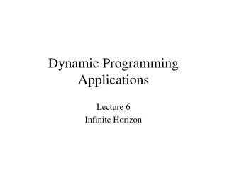
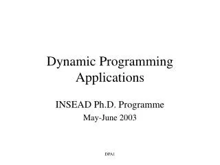
Dynamic Programming Applications. INSEAD Ph.D. Programme May-June 2003. What are we doing here ?. Learning to make long-term decisions …. Today. Introduction Deterministic problems Shortest paths Principle of optimality Deterministic finite state systems & SP

Dynamic Programming Applications
E N D
Presentation Transcript
Dynamic Programming Applications INSEAD Ph.D. Programme May-June 2003 DPA1
What are we doing here ? Learning to make long-term decisions … DPA1
Today • Introduction • Deterministic problems • Shortest paths • Principle of optimality • Deterministic finite state systems & SP • DP vs IP: Knapsack & more .. DPA1
In context • Optimization class: LP/NLP/IP/Networks: static decisions, nothing random or hidden • Contrast: DP = optimize “over time” (*) • Main features: • dynamical systems • stochastic evolution DPA1
Action Action Present state Next state Cost Cost system Sequential decision making model & ingredients DPA1
Planning ahead Present decisions affect future events by: • making certain opportunities available • precluding others • altering costs of still others Trade-off: low cost now vs. high costs in future DP: techniques for making interrelated sequential decisions DPA1
Objective Reflects the decision makers inter-temporal tradeoffs. minimize/maximize • total expected return • total discounted return • average reward per stage • worst case expected return • expected utility • preference ordering • multi-objective (e.g. mean-variance) DPA1
Tools • Decision rule: specifies action to be taken at particular time • Policy: sequence of decision rules; prescription for taking actions in the future. • Optimal policy: policy that optimizes objective. DPA1
Questions • When does an optimal policy exist ? • When does it have a particular form ? • How do we determine or compute efficiently an optimal policy ? • Can we obtain an almost optimal policy, and how good is this? DPA1
Problem Types • finite vs infinite state set • finite vs infinite horizon (epoch set) (L.6-7) • discrete vs continuous time (L.9) • deterministic (Lec.1) vs stochastic system DPA1
Early history • 17th century calculus of variations • Cayley 1875 • Wald: sequential statistical problems 1947 • Pierre Massé 1946: water resource mgt. • RAND Corp., Ca: 1949-1953 • Books: Bellman 1957, Howard 1960 DPA1
B E H A C F J I D G The Stagecoach story • some 150 years ago there was a salesman travelling west by stagecoach .. DPA1
7 1 2 4 4 6 3 B 3 E 6 4 2 H 3 4 4 A C F J 4 3 3 I 1 3 D G 5 Insurance Costs DPA1
The Stagecoach Cont’d • Greedy: A-B-F-I-J costs 13$ • But.. A-D-F = 4 < A-B-F = 6 A-D = 3 > A-B = 2 • not to be greedy pays off! • Trial and error ~ exhaustive enumeration – takes forever! • Idea: Work backwards! DPA1
The Stagecoach Solution • F(X)= min cost from X to J (“cost-to-go”) • F(J)=0 • F(H)=3, F(I)=4 • F(G)=6, F(F)=7, F(E)= 4 • F(D)= 8, F(C )=7, F(B)= 11 • F(A)=11 on A-D-F-I-J (not unique!) DPA1
ut xt xt+1 gt(xt,ut) t t+1 xt+1= f(xt, ut,,t) = ft(xt, ut), t = 0,1,..N-1 state, control, time horizon Deterministic Dynamical System DDS: the state at the next stage is completely determined by state and decision at current stage. DPA1
N-1 t=0 DDP Ingredients • Deterministic dynamic system described by state xt St ( St = state space at time t ). • Control/action to be selected at time t: utUt(xt). (Ut(xt) = action set at time t in state xt). • Dynamics (plant equation): xt+1= ft(xt, ut), t= 0,1,..N-1 • Total cost function: additive over time gN(xN) + S gt(xt,ut) where gt(xt,ut) = cost of decision ut DPA1
Policies • Rule for choosing the value of control variables under all possible circumstances, as a function of perceived circumstances (= strategy, control law) • Actions are taken in real time, whereas a policy is to be formulated in advance. • Closed-loop (or feedback): ut = u(xt, t) sequential decisions depend on the current state • Open-loop control: ut = u*(x0, t) all decisions are made at time t=0 (actions are determined by the clock, as opp. to current state) DPA1
Principle of Optimality • Given the current state, an optimal policy for the remaining stages is independent of the policy adopted in previous stages. • From any point on an optimal trajectory, the remaining trajectory is optimal for the corresp. subproblem initiated at that point. • Action: select a decision to minimize the sum of cost incurred at current stage and least total cost that could be incurred from all subsequent stages, consequent on present decision. DPA1
Bellman’s principle • Jt(xt) = optimal cost starting in state xt at stage t. • Bellman’s principle of optimality: JN(xN) = gN(xN) Jt(xt) = min { gt(xt,ut) + Jt+1(ft (xt,ut)) } “cost-to-go” • Optimal expected cost for overall problem: J0(x0) utUt(xt) DPA1
Deterministic finite state systems • The state space St is finite for each t. • DFS system can be represented by a ‘levelled’ graph of stages, or decision tree. • DFS problem Shortest Path* problem: DPA1
g1(x1,u1) x1 u1 Artificial terminal node Initial state s t Terminal arcs w/cost = terminal cost gN(xN) Stage 0 Stage 1 Stage 2 Stage N DFS SP x2 DPA1
SP DFS • Assume no negative cost cycles ! • So optimal path takes at most N ‘steps’ (allow degenerate steps i i at cost aii=0) • Jk(i) = min cost from i to t in N-k moves • Jk(i) = minj { aij + Jk+1(j)} , k=0,1,..N-2 • JN-1(i) = ait , i=1,2,..N • J0(i) = cost of optimal path from i to t DPA1
Deterministic Applications • Knapsack • Project planning (critical path analysis) DPA1
Knapsack • Squeeze most value in bag of capacity K with objects j=1,…,n of value vj and weight wj. • Vi(w) = max value using some of the first i items and total weight allowed w • Bellman’s equation: Vi+1(w) = max{Vi(w), Vi(w-wi+1) + vi+1} • Boundary conditions ? State set ? • Complexity ? • Interactive applet: http://memento.ieor.berkeley.edu/~jun/knapsack/ DPA1
Project Planning and Critical Path Analysis • Project: K activities of known durations • Some need to be completed before others • Find min completion time & critical activities • nodes = completion of some project phase node 1 = start ; node N = end of project • arc (i, j) =activity that starts once phase i is completed and has duration tij • Acyclic network with all nodes reachable from 1 DPA1
Critical Path Analysis • Path 1 i: p ={ (1,j1), (j1,j2),..,(jk,i)} • Duration: Dp= t(1,j1) + t(j1,j2) + .. + t(jk,i) • Completion of phase i: Ti = max{Dp| paths p: 1 i} • Longest path problem SP(G, -tij) shortest path for graph with negative arc lengths DPA1
Critical Path Analysis • Let Sk={i| all paths: 1 i have k arcs}, S0={1} (nodes reachable in k steps from node 1 ) • Threshold property: k* s.t. Sk=S for all k k*, else SkS. • Shortest path algorithm: Ti = max { tij + Tj}, for all iSk, iSk-1 • Forward DP algorithm (j,i), jSk-1 DPA1
3 order transport end start 2 2 construction 1 1 5 training 4 2 3 4 2 hire training Critical Path Analysis S0={1}, S1={1,2}, S2={1,2,3}, S3={1,2,3,4}, S4={1,2,3,4,5} Completion times: T1=0, T2=3, T3=4, T4=6, T5=10 Critical path: 1 2 3 4 5 DPA1
Fun Applets • GIDEN network animation algorithms http://www.iems.nwu.edu/~giden/download/ • Shortest paths applet http://www.princeton.edu/~rvdb/JAVA/CIV201/shortpaths/shortpaths.html • Knapsack http://memento.ieor.berkeley.edu/~jun/knapsack/ DPA1
Which is the most crucial step ? Guidelines for DP algorithms • View solution as a sequence of decisions occurring in stages and incurring additive costs • Define state as a summary of all relevant past decisions • Determine which state transitions are possible and identify their corresponding costs. • Write a recursion on the optimal cost from the origin state to a destination state DPA1
To Remember • The optimal ut is only a function of state xt & time t • The DP equation expresses the optimal ut in closed loop form. It is optimal whatever the past control policy may have been. • The DP equation is backward induction in time; always the later policy is decided first. • Determ. FS. DP Shortest Path w/o neg. cycles Read Bkas Chapter 2 DPA1