Session 3 Analysis of mediation and moderation using instrumental variables Richard Emsley

MethodologyResearch Group Methods of explanatory analysis for psychological treatment trials workshop Session 3 Analysis of mediation and moderation using instrumental variables Richard Emsley Funded by: MRC Methodology GrantG0600555 MHRN Methodology Research Group

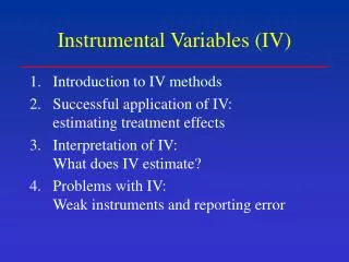
Plan for session 3 • Quick review of instrumental variables from Ian’s talk. • Why do we use instrumental variables? • Where do we find instrumental variables? • Examples: • PROSPECT mediator example • SoCRATES S+A*S model. • Designing trials with instruments in mind.

Quick review of IVs from Ian’s talk… • Ian has demonstrated how we can use instrumental variable methods to infer a causal effect of treatmentin the presence of departures from randomised intervention. • This utilises randomisation as the instrumental variable. As we will see, randomisation meets the assumptions required for an IV… • But we will also need to consider the situation where we cannot use randomisation as an instrument…

Instrumental Variables (IVs) • In a standard regression model, if an explanatory variable is correlated with the error term (known as endogeneity) its coefficient cannot be unbiasedly estimated. • An instrumental variable (IV) is a variable that does not appear in the model, is uncorrelated with the error term and is correlated with the endogenous explanatory variable; randomisation, where available, often satisfies this criteria. • A two stage least squares (2SLS) procedure can then be applied to estimate the coefficient. At its simplest, the first stage involves using a simple linear regression of the endogenous variable on the instrument and saving the predicted values. In the second stage the outcome is then regressed on the predicted values, with the latter regression coefficient being the required estimate of the coefficient.

Some notation • Ri – treatment group: the outcome of randomisation (Ri=1 for treatment, 0 for controls). • Xi′ = X1i, X2i … Xpi – baseline covariates. • Yi – observed outcome. • Di – actual treatment received. This is an intermediate outcome that is a putative mediator of the effects of treatment on outcome (either a quantitative measure or binary).

Instrumental variables (IV) (from session 1) • Popular in econometrics • Simplest idea is: • Outcome: Yi = a + b Di + ei • Treatment: Di = g + d Ri + fi • Allow error ei to be correlated with Di but assume it’s independent of Ri • randomisation Ri only affects outcome through its effect on compliance Di • Estimation by “two-stage least squares”: • E[Yi | Ri] = a + b E[Di | Ri] • so first regress Di on Ri to get E[Di | Ri] • then regress Yi on E[Di | Ri] • NB standard errors not quite correct by this method: general IV uses different standard errors

Simple Mediation Idea (from session 2) dX Mediator β α Treatment Outcomes dY γ The total effect is the sum of the direct effect (γ) and the indirect effect (α*β)

Confounded Mediation Diagram U – the unmeasured confounders dX U Mediator β α Treatment Outcomes dY γ If treatment is randomised then assumption of no confounding of treatment and other variables (outcomes) is justified.

Confounded Mediation Diagram dX U U Mediator β α Treatment Outcomes dY γ U If treatment is not randomised then there is likely to be even more unmeasured confounding.

Confounded Mediation Diagram dX U Mediator β α Randomisation Outcomes dY γ Thankfully we’re talking about randomised trials!

Linking the two previous sessions: Compliance as a mediator dX Treatment Received Randomisation Outcomes dY

Linking the two previous sessions: Randomisation as an IV dX Treatment Received Randomisation Outcomes dY By assuming the absence of a direct path from randomisation to outcome, we assume the entire effect of randomisation acts through receipt of treatment. → randomisation is an instrumental variable.

Why do we use instrumental variables? • All available statistical methods we usually use (for any standard analysis), including: • Stratification • Regression • Matching • Standardization • require the one unverifiable condition we identified previously: NO UNMEASURED CONFOUNDING

Why do we use instrumental variables? • Unlike all other methods, IV methods can be used to consistently estimate causal effects in the presence of unmeasured confounding AND measurement error. • SO WE CAN SOLVE THE PROBLEM OF… dX U Mediator β α Randomisation Outcomes dY γ

Definition of an instrumental variable A variable is an instrumental variable Z if: • Z has a causal effect on the mediator D; This can be tested in the data. ii. Z affects the outcome Y only through D i.e. there is no direct effect of Z on Y; This is an assumption (sometimes a strong assumption). iii. Z does not share common causes with the outcome Y i.e. there is no confounding for the effect of Z on Y. This is another assumption which randomisation satisfies but other IVs may not.

Assumptions for instrumental variables • IV methods require FOUR assumptions • The first 3 assumptions are from the definition: • The association between instrument and mediator. • no direct effect of the instrument on outcome. • no unmeasured confounding for the instrument and outcome. • There are a wide variety of fourth assumptions and different assumptions result in the estimation of different causal effects: • E.g. no interactions, monotonicity (no defiers).

Testing assumptions… • There are a number of tests we can use for some of these assumptions. • Stata has three postestimation commands following ivregress: • estat overid • estat endogenous • estat firststage • This final option is perhaps the most useful. It gives an indication of whether the set of instruments strongly predict the mediator – see PROSPECT example later on.

Advantages of IVs • Can allow for unmeasured confounding; • Can allow for measurement error; • Randomisation meets the definition so is an ideal instrument • When available. • Obviously not in observational studies.

Disadvantages of IVs 1. It is impossible to verify that Z is an instrument and using a non instrument introduces additional bias. 2. A weak instrument Z increases the bias over that of ordinary regression. 3. Instruments by themselves are actually insufficient to estimate causal effects and we require additional unverifiable assumptions such as the “no defiers” assumption. 4. Standard IV methods do not cope well with time-varying exposures/mediators…yet. See Hernán and Robins (2006), Epidemiology for further details

Assumption trade-off • IV methods replace one unverifiable assumption of no unmeasured confounding between the mediator and the outcome by other unverifiable assumptions • no unmeasured confounding for the instruments, or • no direct effect of the instruments. • We need to decide which assumptions are more likely to hold in our mediation analysis. • An IV analysis will also increase the precision of our estimates because of allowing for the unmeasured confounding.

Also… • What about if we want to estimate the direct effect of randomisation in the presence of a potential mediator? dX U Mediator β α Randomisation Outcomes dY γ Clearly we can’t use randomisation as an instrument here…we need another instrument.

Multiple instruments • When we are trying to estimate the direct effect of randomisation we need alternative instruments. • Likewise, if we have more than one endogenous variable (multiple mediators), then we need multiple instruments. • For IV model identification, we always need to have as many instruments as we have endogenous variables. • i.e. if considering two mediators in the model (therapeutic alliance and number of sessions of therapy attended), then we need at least two instrumental variables.

Where do we find instruments? • Possibilities for IVs: • Randomisation-by-baseline variable interactions. • Randomisation involving more than one active treatment – i.e. to interventions specifically targeted at particular intermediate variables/mediators. • Randomisation-by-trial (multiple trials). • Genetic markers (Mendelian Randomisation) used together with randomisation.

Confounded Mediation Diagram U – the unmeasured confounders dX U Mediator β α Randomisation Outcomes dY γ If treatment is randomised then assumption of no confounding of treatment and other variables (outcomes) is justified.

Mediation Diagram with instruments U – the unmeasured confounders dX U Randomisation*Covariates Mediator β α Randomisation Outcomes dY γ Covariates

Multiple Instruments • Here, treatment by covariates interactions represent instrumental variables. • Assumptions: • The interactions are significant in the first stage regression (individually and joint F-test). • The only effect of the interactions on outcome is through the mediator, and not a direct effect. This is a very strong assumption • No other unmeasured confounders between the interactions and outcome.

Summary so far… • The analysis of mediation is more complex than it first seems because of potential unmeasured confounding (mediators are endogenous). • We use moderators of the relationship between randomisation and the mediator (i.e. the baseline by randomisation interactions) as instruments. • The analysis of mediation by instrumental variables requires additional assumptions. Primarily, that these covariates are not moderators of the randomisation on outcome relationship (no direct effect). • We illustrate these points on two examples now…

Example: PROSPECT • PROSPECT (Prevention of Suicide in Primary Care Elderly: Collaborative Trial) was a multi-site prospective, randomised trial designed to evaluate the impact of a primary care-based intervention on reducing major risk factors (including depression) for suicide in elderly depressed primary care patients. • The two conditions were either: • (a) an intervention based on treatment guidelines tailored for the elderly with care management, • (b) treatment as usual. • An intermediate outcome in the PROSPECT trial was whether the trial participant adhered to antidepressant medication during the period following allocation of the intervention. • The question here is whether changes in medication adherence following the intervention might explain some or all of the observed (ITT) effects on clinical outcome. See Bruce et al, JAMA (2004); Ten Have et al, Biometrics (2007); Bellamy et al, Clinical Trials (2007); Lynch et al, Health Services and Outcome Research Methodology (2008). Thanks to Tom Ten Have for use of the data.

Example: PROSPECT - question of interest Randomisation*Covariates Antidepressant Use Depression Score Randomisation Covariates

Example: PROSPECT - summary stats

PROSPECT data – Stata describe . describe Contains data from P:\SMinMR paper\Prospect.dta obs: 297 vars: 8 11 Sep 2009 16:01 size: 20,196 (99.9% of memory free) -------------------------------------------------------------------------------------------- storage display value variable name type format label variable label -------------------------------------------------------------------------------------------- cad1 double %10.0g Anti-depressant use at baseline visit hdrs0 double %10.0g Hamilton depression score at baseline visit ssix01 double %10.0g Suicide ideation at baseline visit scr01 double %10.0g Past medication use at baseline visit hdrs4 double %10.0g Hamilton depression score at 4 month visit site double %10.0g Location of practices interven double %10.0g Randomized assignment to intervention Amedx double %10.0g Adherence to prescribed anti-depressant medication --------------------------------------------------------------------------------------------

PROSPECT data – Stata ivregress . xi: ivregress 2sls hdrs4 hdrs0 cad1 ssix01 scr01 i.site i.interven (amedx = i.interven*hdrs0 i.interven*cad1 i.interven*ssix01 i.interven*scr01 i.interven*i.site), first First-stage regressions -------------------- Number of obs = 296 F( 13, 282) = 21.71 Prob > F = 0.0000 R-squared = 0.5002 Adj R-squared = 0.4772 Root MSE = 0.3465 ------------------------------------------------------------------------------ amedx | Coef. Std. Err. t P>|t| [95% Conf. Interval] -------------+---------------------------------------------------------------- hdrs0 | .0065731 .0051473 1.28 0.203 -.0035588 .0167051 cad1 | .166495 .0254223 6.55 0.000 .1164533 .2165366 ssix01 | -.0475454 .0721387 -0.66 0.510 -.1895441 .0944533 scr01 | .2530611 .0746616 3.39 0.001 .1060962 .4000259 _Isite_2 | -.018463 .0664307 -0.28 0.781 -.149226 .1123 _Isite_3 | .1969925 .0734302 2.68 0.008 .0524516 .3415334 _Iinterven_1 | .7825965 .1398924 5.59 0.000 .5072307 1.057962 _IintXhdrs~1 | -.003633 .0071484 -0.51 0.612 -.0177041 .010438 _IintXcad1_1 | -.118277 .0341169 -3.47 0.001 -.1854331 -.0511209 _IintXssix~1 | .0504564 .0967541 0.52 0.602 -.1399956 .2409083 _IintXscr0~1 | -.2627584 .1029091 -2.55 0.011 -.4653259 -.0601909 _IintXsit_~2 | -.0099335 .095321 -0.10 0.917 -.1975645 .1776975 _IintXsit_~3 | -.1681695 .1054282 -1.60 0.112 -.3756956 .0393566 _cons | -.0465641 .0996531 -0.47 0.641 -.2427223 .1495942 ------------------------------------------------------------------------------

PROSPECT data – Stata ivregress Instrumental variables (2SLS) regression Number of obs = 296 Wald chi2(8) = 102.68 Prob > chi2 = 0.0000 R-squared = 0.2582 Root MSE = 6.8425 ------------------------------------------------------------------------------ hdrs4 | Coef. Std. Err. z P>|z| [95% Conf. Interval] -------------+---------------------------------------------------------------- amedx | -1.95302 2.672201 -0.73 0.465 -7.190438 3.284397 hdrs0 | .6226062 .070337 8.85 0.000 .4847482 .7604642 cad1 | -.0654087 .4304821 -0.15 0.879 -.9091381 .7783208 ssix01 | 1.251204 .9399736 1.33 0.183 -.5911102 3.093518 scr01 | 1.585044 1.074312 1.48 0.140 -.5205695 3.690658 _Isite_2 | -.4971475 .9469522 -0.52 0.600 -2.35314 1.358845 _Isite_3 | -2.046048 1.08319 -1.89 0.059 -4.169062 .0769655 _Iinterven_1 | -2.375598 1.328982 -1.79 0.074 -4.980353 .2291584 _cons | 3.344043 1.467043 2.28 0.023 .4686928 6.219394 ------------------------------------------------------------------------------ Instrumented: amedx Instruments: hdrs0 cad1 ssix01 scr01 _Isite_2 _Isite_3 _Iinterven_1 _IintXhdrs0_1 _IintXcad1_1 _IintXssix0_1 _IintXscr01_1 _IintXsit_1_2 _IintXsit_1_3

Example: PROSPECT - results Using all baseline variables as covariates in an ANCOVA. ITT effect: -3.15 (0.82) Small but statistically significant effect Direct effect Indirect effect γ (s.e.) β (s.e.) Analytical method Standard regression -2.66 (0.93) -1.24 (1.09) (Baron & Kenny)

Example: PROSPECT - results Direct effect Indirect effect γ (s.e.) β (s.e.) Analytical method IV (ivreg) -2.38 (1.35) -1.95 (2.71) IV (treatreg - ml) -2.34 (1.27) -2.05 (2.49) G-estimation* -2.58 (1.27) -1.43 (2.34) Conclusion Allowing for hidden confounding appears to have had little effect, except to increase the SE of the estimate. *From Ten Have et al, Biometrics (2007)

PROSPECT data – ivregress postestimation . estat firststage First-stage regressions -------------------- Number of obs = 296 F( 13, 282) = 21.71 Prob > F = 0.0000 R-squared = 0.5002 Adj R-squared = 0.4772 Root MSE = 0.3465 ------------------------------------------------------------------------------ amedx | Coef. Std. Err. t P>|t| [95% Conf. Interval] -------------+---------------------------------------------------------------- hdrs0 | .0065731 .0051473 1.28 0.203 -.0035588 .0167051 cad1 | .166495 .0254223 6.55 0.000 .1164533 .2165366 ssix01 | -.0475454 .0721387 -0.66 0.510 -.1895441 .0944533 scr01 | .2530611 .0746616 3.39 0.001 .1060962 .4000259 _Isite_2 | -.018463 .0664307 -0.28 0.781 -.149226 .1123 _Isite_3 | .1969925 .0734302 2.68 0.008 .0524516 .3415334 _Iinterven_1 | .7825965 .1398924 5.59 0.000 .5072307 1.057962 _IintXhdrs~1 | -.003633 .0071484 -0.51 0.612 -.0177041 .010438 _IintXcad1_1 | -.118277 .0341169 -3.47 0.001 -.1854331 -.0511209 _IintXssix~1 | .0504564 .0967541 0.52 0.602 -.1399956 .2409083 _IintXscr0~1 | -.2627584 .1029091 -2.55 0.011 -.4653259 -.0601909 _IintXsit_~2 | -.0099335 .095321 -0.10 0.917 -.1975645 .1776975 _IintXsit_~3 | -.1681695 .1054282 -1.60 0.112 -.3756956 .0393566 _cons | -.0465641 .0996531 -0.47 0.641 -.2427223 .1495942 ------------------------------------------------------------------------------

PROSPECT data – ivregress postestimation (no endogenous regressors) ( 1) _IintXhdrs0_1 = 0 ( 2) _IintXcad1_1 = 0 ( 3) _IintXssix0_1 = 0 ( 4) _IintXscr01_1 = 0 ( 5) _IintXsit_1_2 = 0 ( 6) _IintXsit_1_3 = 0 F( 6, 282) = 9.10 Prob > F = 0.0000 First-stage regression summary statistics -------------------------------------------------------------------------- | Adjusted Partial Variable | R-sq. R-sq. R-sq. F(6,282) Prob > F -------------+------------------------------------------------------------ amedx | 0.5002 0.4772 0.1622 9.10057 0.0000 -------------------------------------------------------------------------- Minimum eigenvalue statistic = 9.10057 Critical Values # of endogenous regressors: 1 Ho: Instruments are weak # of excluded instruments: 6 --------------------------------------------------------------------- | 5% 10% 20% 30% 2SLS relative bias | 19.28 11.12 6.76 5.15 -----------------------------------+--------------------------------- | 10% 15% 20% 25% 2SLS Size of nominal 5% Wald test | 29.18 16.23 11.72 9.38 LIML Size of nominal 5% Wald test | 4.45 3.34 2.87 2.61 ---------------------------------------------------------------------

Instrumental Variables in SPSS Analyse – Regression – 2-stage Least Squares Generate interactions as additional variables using compute

Instrumental Variables in SPSS Outcome Covariates and endogenous variable (mediator) Covariates and instruments

Example: the SoCRATES trial • SoCRATES was a multi-centre RCT designed to evaluate the effects of cognitive behaviour therapy (CBT) and supportive counselling (SC) on the outcomes of an early episode of schizophrenia. • 201 participants were allocated to one of three groups: • Control: Treatment as Usual (TAU) • Treatment: TAU plus psychological intervention, either CBT + TAU or SC + TAU • The two treatment groups are combined in our analyses • Outcome: psychotic symptoms score (PANSS) at 18 months

Example: SoCRATES - summary stats Lewis et al, BJP (2002); Tarrier et al, BJP (2004); Dunn & Bentall, Stats in Medicine (2007); Emsley, White and Dunn, Stats Methods in Medical Research (2009).

Confounded Dose-Response dX U Sessions Attended β α Randomisation Psychotic Symptoms dY Are the effects of Randomisation on Sessions (α) and, more interestingly, the effects of Sessions on Outcome (β), influenced by the strength of the therapeutic alliance?

The S + A*S model • We want to estimate the joint effects of the strength of the therapeutic alliance as measured by CALPAS (A) and number of sessions attended (S). • We postulate a structural model as follows: E[Yi(1)-Yi(0)| Xi, Di(1)=s, Di(0)=0 & Ai=a] = βs*s + βsa*s*(a-7) • No sessions implies no treatment effect. • The effect of alliance is multiplicative so we only have an interaction effect of alliance – no sessions = no alliance. Dunn and Bentall, SiM (2007)

SoCRATES analysis results Method βs (se) βsa (se) Instrumental variables -2.40 (0.70) -1.28 (0.48) Standard regression (B&K) -0.95 (0.22) -0.39 (0.11) Note: A has been rescaled so that maximum=0. When A=0 (i.e. maximum alliance) the slope for effect of Sessions is -2.40 When A=-7 (i.e. minimum alliance) the slope is -2.40 + 7*1.28 = +6.56 This suggests that when alliance is very poor attending more sessions makes the outcome worse!

SoCRATES – S + A*S using regress . regress pant18 sessions s_a pantot logdup c1 c2 yearsed Source | SS df MS Number of obs = 153 -------------+------------------------------ F( 7, 145) = 15.78 Model | 24414.5544 7 3487.79349 Prob > F = 0.0000 Residual | 32051.4194 145 221.044272 R-squared = 0.4324 -------------+------------------------------ Adj R-squared = 0.4050 Total | 56465.9739 152 371.48667 Root MSE = 14.868 ------------------------------------------------------------------------------ pant18 | Coef. Std. Err. t P>|t| [95% Conf. Interval] -------------+---------------------------------------------------------------- sessions | -.9459469 .2209236 -4.28 0.000 -1.382593 -.5093003 s_a | -.3866447 .1117784 -3.46 0.001 -.6075702 -.1657192 pantot | .3843765 .087454 4.40 0.000 .2115272 .5572259 logdup | 2.331363 2.398488 0.97 0.333 -2.409152 7.071878 c1 | 4.322976 3.48805 1.24 0.217 -2.571014 11.21697 c2 | -11.96141 3.292382 -3.63 0.000 -18.46867 -5.454147 yearsed | -1.110149 .5318061 -2.09 0.039 -2.161242 -.0590559 _cons | 43.94059 11.21352 3.92 0.000 21.77752 66.10366 ------------------------------------------------------------------------------

SoCRATES – S + A*S using ivregress . ivregress 2sls pant18 pantot logdup c1 c2 yearsed (sessions s_a = group lgp c1gp c2gp yrgp pgp) First-stage regressions ----------------------- Number of obs = 153 F( 11, 141) = 78.68 Prob > F = 0.0000 R-squared = 0.8599 Adj R-squared = 0.8490 Root MSE = 3.3588 ------------------------------------------------------------------------------ sessions | Coef. Std. Err. t P>|t| [95% Conf. Interval] -------------+---------------------------------------------------------------- pantot | 1.71e-14 .0310634 0.00 1.000 -.0614103 .0614103 logdup | 2.46e-13 .858628 0.00 1.000 -1.697449 1.697449 c1 | -3.59e-13 1.125814 -0.00 1.000 -2.225657 2.225657 c2 | 4.70e-14 1.022741 0.00 1.000 -2.021889 2.021889 yearsed | 1.17e-13 .1929797 0.00 1.000 -.3815077 .3815077 group | 16.09465 5.201659 3.09 0.002 5.811326 26.37798 lgp | .1800265 1.104039 0.16 0.871 -2.002583 2.362636 c1gp | -1.281224 1.574428 -0.81 0.417 -4.39376 1.831312 c2gp | -3.772746 1.471898 -2.56 0.011 -6.682588 -.8629052 yrgp | .1835663 .2475856 0.74 0.460 -.3058935 .6730261 pgp | -.0104563 .0407688 -0.26 0.798 -.0910534 .0701407 _cons | -3.05e-12 4.115125 -0.00 1.000 -8.135319 8.135319 ------------------------------------------------------------------------------ Model for sessions

SoCRATES – S + A*S using ivregress Number of obs = 153 F( 11, 141) = 16.59 Prob > F = 0.0000 R-squared = 0.5641 Adj R-squared = 0.5301 Root MSE = 12.0225 ------------------------------------------------------------------------------ s_a | Coef. Std. Err. t P>|t| [95% Conf. Interval] -------------+---------------------------------------------------------------- pantot | -1.89e-14 .1111878 -0.00 1.000 -.2198106 .2198106 logdup | -1.89e-13 3.073353 -0.00 1.000 -6.075809 6.075809 c1 | 3.31e-13 4.029712 0.00 1.000 -7.966465 7.966465 c2 | -3.78e-14 3.660775 -0.00 1.000 -7.237101 7.237101 yearsed | -1.00e-13 .6907472 -0.00 1.000 -1.36556 1.36556 group | -16.2085 18.6187 -0.87 0.385 -53.0164 20.59939 lgp | -6.186983 3.951771 -1.57 0.120 -13.99936 1.625398 c1gp | -11.44637 5.635471 -2.03 0.044 -22.58731 -.3054279 c2gp | -4.923988 5.268477 -0.93 0.352 -15.33941 5.49143 yrgp | -.1321276 .8862022 -0.15 0.882 -1.884089 1.619833 pgp | .0765408 .1459268 0.52 0.601 -.2119464 .3650281 _cons | 2.96e-12 14.72958 0.00 1.000 -29.11937 29.11937 ------------------------------------------------------------------------------ Model for sessions*alliance

Session 3 Analysis of mediation and moderation using instrumental variables Richard Emsley