Download
1 / 18
180 likes | 341 Views
Computational Intelligence: Methods and Applications. Lecture 32 Nearest neighbor methods Włodzisław Duch Dept. of Informatics, UMK Google: W Duch. k-NN .

E N D
Computational Intelligence: Methods and Applications Lecture 32 Nearest neighbor methods Włodzisław Duch Dept. of Informatics, UMK Google: W Duch
k-NN k-Nearest Neighbors method belongs to the class of “lazy” algorithms – all work (or most work) is done during the query time, while other algorithms model the data at the training stage. Very simple idea: find k most similar cases to X and claim that X is like majority of these cases. It is so important that in different branches of science and applications it is known under many names: • Instance-Based Methods (IBM), or Instance Based Learning (IBL) • Memory-Based Methods (MBM), • Case-Based Methods (CBM), • Case-Based Reasoning (CBR), • Memory-Based Reasoning (MBR), • Similarity-Based Reasoning (SBR), • Similarity-Based Methods (SBM)
Non-parametric density again Histograms and Parzen windows are one way to evaluate PDF in low-dimensional spaces, but these windows may be defined in d dimensions around some data vector. Probability P that a data point comes from some region R (belongs to some category etc) is: If this probability does not change in a small volume of space too much then P(X) VRP = k/n, where k is the number of samples found in the volume VRand n the number of all samples. In histogram approach the size (here volume) is fixed, and k changes. Fix k, then P(X) ~ 1/VRor the volume which contains k samples. Find a sphere with center at X that contains k samples; Bayesian decision: select the class which is most often represented.
Bayesian justification Let the total number of samples from class wcbe n(wc) and the number of sample in volume V from class wcbe k(wc). For K classes they sum to: Estimate of class-conditional density is: and the prior probability: and the density: so the posterior probability: P(X) is not needed for Bayes rule.
MAP decision Maximum a posteriori (MPA) Bayesian decision is equivalent to: because using Bayes formula: MAP Bayesian decision says: given k nearest neighbors of sample X, assign X to the class wc that the majority of samples belong to. This is a theoretical basis for a family of nearest-neighbor methods.
kNN decision borders All training vectors D={X(i)}, i=1..n, are used as reference; finding one nearest neighbor creates Voronoi tessellation of the feature space; resulting decision borders are piecewise linear, but quite complex. Here red samples create a strange polyhedral figure – any vector that is inside will be assigned to the red class. Duda et al, Fig. 4.13 For k > 1 decision borders are smoother and small disconnected regions will vanish. Recall that larger k corresponds to larger volume or larger widows in the density estimation procedure. See applet here.
Theoretical results 1-NN error rate for infinite number of training samples is bounded by: The proof is rather long (see Duda et al, 2000). Thus the error of 1-NN is not larger than twice the Bayes error. For both k and n going to infinity k-NN error converges to Bayesian, but in practice optimal k should be selected for the given data. Good news: Select X(i), find its k neighbors and classify it Report average accuracy This is the leave-one-out error! We remove a single vector and use the rest to predict is class. Usually it is very expensive to calculate.
Complexity Time required for a single vector classification is O(dn). Evaluation of error requires O(dn2) operations.Too slow for real-time applications, discrimination methods are faster. Solutions (there are more): 1) Parallel implementation may reduce time for a single vector to O(1). Voronoi cell has m planes: each cell is represented by munits that check if X is inside or outside the plane; AND unit combines results and assigns X to a cell. 2) All training vectors are taken as reference vectors, but there is no need to use that many, only vectors that are near the decision border are important – this is known as editing, pruning or condensing. Discard all X(i) with all adjacent Voronoi regions from the class of X(i)
Subtle points Parameter k may be selected by calculating the error with k=1 .. kmax Careful ... this is good k for calculation on some test data, but since all data has been used for parameter selection, this is not an estimation of expected error! Taking one vector out, optimal k should be determined calculating error on the remaining n-1 vectors; optimal k may be different for the next vector. The differences are small in practice. kNN is stable! Small perturbation of training data does not change results significantly. This is not true for covering methods, decision trees etc. Breaking ties: what if k=3, and neighbor is from different class? Use P(w|X)=1/3, or find additional neighbor, or select the closest, or the one from most common class, or break the tie randomly, or ...
Distance functions “Nearest” in what sense? A distance function evaluates dissimilarity. Most distance functions are a sum of feature dissimilarities: This is called Minkovsky distance function.The exponent allows to change the shapes of D(X,0)2=||X||2 The simplest feature dissimilarity is: di(Xi,Yi) = |Xi-Yi| for real-valued features di(Xi,Yi) = d(Xi,Yi)for binary, logical or nominal features this is called overlapped difference For real-valued features distance may be divided by a normalization factor, such as q = max(Xi)–min(Xi) or q=4si
Popular distance functions Minkovsky distance from 0: for a = 1/2, 1, 2, and 10 Minkovsky distance functions are also called La norms Manhattan distance or L1 norm: Guess why this is called “Manhattan” or “a city block” metrics? Euclidean distance or L2 norm: Natural in Euclidean spaces, no need to take the square root comparing distances.
Normalization, scaling and weighting Distance depends on the units, therefore features should be normalized: The relative importance of features may be expressed by setting the scaling factor Sj =1 for the most important feature, and other scaling factors to the desired ones. Scaling factors may be optimized by minimization of the number of errors that the kNN classifier makes. Should all knearest neighbors be counted with the same weight? Posterior probability is ~ a sum of contributions of some distance-dependent factors h(D)=exp(-D), or h(D)=1/D. BelowC(R) is the true class, and k may be relatively large (in RBF networks k=n).
Some advantages Many! One of the most accurate methods, for example in image classification problems (see Statlog report). • Does not need the vectors, only distance matrix! Therefore complex objects with internal structures may be compared. • No restriction to the number of classes; prediction of real-valued outputs is done using kNN by combining locally weighted values assigned to reference vectors => Locally Weighted Regression. • Instead of class labels vector outputs may be used, forming associations between input and output vectors. • Prediction may be done in subspaces, skipping the missing values, or determining most probable missing values using the remaining information. • Simple to implement, stable, no parameters (except for k), easy to run leave-one-out test. • Should be used before more sophisticated methods.
Few disadvantages Not that many, but ... • Needs relatively large data sets to make reliable predictions. • Small k solutions may introduce rugged borders and many disjoint areas assigned to one class; if k=1 is optimal and significantly better than other k there may be some problem with the data ... • Relatively large memory requirements for storage of the distance matrix, O(n2) unless condensing is used. • Slow during classification, used only in off-line applications. • Depends on the scaling of features, but normalization does not always helps (decision trees of LDA do not require that) • Sensitive to noise in features – if many noisy features are present distances may be useless. • Not easy to interpret if the reference set of vectors is large and distance functions involve all dimensions. • Warning: 1-NN result on the training set are 100% - use always crossvalidation or leave-one-out for estimation.
IBk in WEKA Instance Base k-neighbors, is the k-NN implementation in WEKA. • k: number of nearest neighbors to use in prediction (default 1) • W: Set a fixed window size for incremental train/testing. As new training instances are added, oldest instances are removed to maintain the number of training instances at this size. • D: Neighbors will be weighted by the inverse of their distance when voting (default: equal weighting). • F: Neighbors will be weighted by their similarity (1-D/Dmax) when voting (default: equal weighting). • X: Selects the number of neighbors to use by the leave-one-out method, with an upper limit given by the -k option. • S: When k is selected by cross-validation for numeric class attributes, minimize mean-squared error (default mean absolute error).
IB1 and IBk examples Simplest implementation in WEKA: IB1. k=1, Euclidean distance, no editable properties, does normalization. Credit-Australia data: should a bank give credit to a customer or not? 15 features, 690 samples, 307 in class +, 383 in class -. GM: IB1 style: 64.5±8.3 raw data, 80.9±3.6 normalized. IB1 gives 81.2% correct predictions in 10xCV; confusion matrix is: a b <= classified as 239 68 | a = + 62 321 | b = - IBk k=1..10, selected k=7 as optimal, accuracy 87.0% (±? not easy). GM: k=1..10, with k=7, 85.8±4.9%, but k=6-9 in different runs. But ... a rule: IF A9=T then class +, A9=F then class -, has Acc=85.5%
Other kNN packages kNN is not so popular as SVM or NN so it is much harder to get good non-commercial software. Similarity Based Learner, software with many options, free from Dr Karol Grudzinski, karol.grudzinski@wp.pl kNN in Ghostminer: autoselection of k, feature weighting. Similarity may sometimes be evaluated by people, and displayed in graphical form: take a look at similarity of music groups: www.liveplasma.com www.pandora.com creates radio stations on demand (tylko USA) Podobne podobne usługi. Demo: pronunciation of English words. Good recent book, wit great chapters on visualization: E. Pekalska & R.P.W. Duin, The dissimilarity representation for pattern recognition: foundations and applications, World Scientific 2005.
More links Editing the NN rule (selecting fewer references), with some applets. A Library forApproximate Nearest Neighbor Searching (ANN) http://www.cs.umd.edu/~mount/ANN/