Download
1 / 36
390 likes | 632 Views
Coupling of compressible and incompressible fluids. Veronika Schleper Institute for Applied Analysis and Numerical Simulation University of Stuttgart joint work with Sino-German Symposium on Advanced Numerical Methods for Compressible Fluid Mechanics and Related Problems

E N D
Coupling of compressible and incompressible fluids Veronika Schleper Institute for Applied Analysis and Numerical Simulation University of Stuttgart joint work with Sino-German Symposium on Advanced Numerical Methods for Compressible Fluid Mechanics and Related Problems Beijing, Mai 22 – 26, 2014
Outline • A compressible two fluid Model • Analytical Results • Well-posedness for all liquid sound speeds • The zero-Mach limit • Numerical Examples • One dimensional test case • Two dimensional algorithm and validation
Example 1: Shock-droplet interaction • Schlieren-type image of a shock interaction with a weakly compressible droplet. Black: high density gradient. Light gray: low density gradient. • [Simulation: joint work with Stefan Fechter, Institute of Aero- and Gasdynamics, University of Stuttgart] t=1.5ms t=1.0ms t=2.5ms 3
A simple model for compressible two-fluid flow • Isothermal Euler equations in gas and liquid: • Here: density, velocity, • pressure law (for gas and liquid) • General assumptions: • Sharp interface • No exchange of mass across the interface, i.e. conservation of mass of liquid and gas phase separately • Isothermal description is sufficient • No occurrence of vacuum states Gas Gas Liquid 4
A simple model for compressible two-fluid flow • Interface conditions in normal direction: • Rankine-Hugoniot jump conditions • Additional assumption (kinetic relation) • All together we have: Gas Gas Liquid 5
The two-fluid Cauchy problem (1D) • For: • For • At the interfaces and : • Initial conditions: Gas Liquid Gas 6
The interface Riemann problem • Definition: For a given initial condition • solves the interface Riemann problem if it coincides for all with • 1. a 1-Lax curve of the -system connecting and • 2. a 2-Lax curve of the -system connecting and • 3. Such that the states and satisfy Well-posedness:Under standard assumptions exists a well-posed local solution. (see Colombo & Schleper, NoRWA 2012) 7
The two-fluid Cauchy problem for arbitrary large (1D) • Definition: Solution of the two-fluid Cauchy problem [Colombo, Schleper 2012] • Let and fix a gas state and a liquid state . • Define . • Choose pressure laws , such that • . • A solution to the compressible two-fluid Cauchy problem is a map • such that • 1. is a weak entropy solution in the gas phase in . • 2. is a weak entropy solution in the liquid phase . • 3. For almost every , the conditions at the interface are satisfied. 10
The two-fluid Cauchy problem for arbitrary large (1D) • Theorem: Well-posedness & the Limit [Colombo, Guerra, Schleper 2013] • For a suitable pressure law and , we have • 1. A set of initial data , such that the compressible Cauchy problem is well-posed for all sufficiently large . • 2. is incompressible, i.e. and are constant. • 3. For any , the solution converges to a solution of the compressible-incompressible system. • 4. The density converges in to , constant in time and space • 5. The velocity converges in to , constant in space • 6. The pressure converges weak* in . 11
The compressible-incompressible system (1D) • For: • At the interface and : • For : • Coupling of pde and ode 12
The compressible-incompressible system (1D) • For: • At the interface and : • For : • Coupling of pde and ode Implicit discretization: 13
The compressible-incompressible system (1D) • For: • At the interface and : • For : • Coupling of pde and ode Implicit discretization: Explicit discretization: 14
Numerical Example (1D) • Several waves hit a 1D droplet initially in equilibrium with surrounding gas. • Pressure laws: • Gas: Liquid: • Initial conditions: • Gas left: • Liquid: • Gas right: Evolution of the pressure for reflective left boundary. Top: incompressible, bottom: compressible. 15
Numerical Example (1D) • Computational effort: • Speed-up depends on: • Number of interfaces / number of drops • Concrete numerical coupling method • Ratio between gas and liquid sound speed • Size of the droplets (only in 2D and 3D) 17
Numerical Example (2D) • Schematic 2D setting: • Coupling of all liquid cells through • Interface condition: • Coupling of all interface cells with all liquid cells • Problem is no longer local 18
Numerical Example (2D) • 2D-Algorithm: • Incompressible region: Approximate projection method • Fractional step method, proposed by Almgren, Bell, Szymczak (1996) • Convection step for the velocity • Projection step assures divergence free velocity field and defines pressure • Compressible region: Finite Volume method • Interface tracking • Advantage: Fractional step method naturally allows for explicit coupling • Convection step: pressure gradients and interface data yield . • Projection step yields and and interface velocity . • (approximate) Lax curves yield at the interface from and . • FV-scheme yields . 19
Conclusion • Analytical justification of an abstract coupling idea in one space dimensions • Numerical approximations of the coupling are well-posed • Implicit and explicit approximations of the coupling conditions work (in first order code) • First 2D results coincide very well with 1D results • Outlook • Validation against fully compressible scheme • Coupling conditions for two-phase flows • Abstract code coupling • Substitute incompressible Euler by incompressible Navier-Stokes • Criteria for model adaptivity (?) 22
Problem formulation in Lagrangian coordinates • For: • For • At the interfaces and : • Initial conditions: • Advantage: Interfaces are stationary. Gas Liquid Gas 23
Problem formulation in Lagrangian coordinates • Additional assumption: • Fix initial specific volume of the liquid. • Special pressure law in the liquid phase: • Hereby: Eulerian sound speed • Lagrangian sound speed • First step: Existence result for arbitrary large . • Second step: Limit . 24
The two-fluid Cauchy problem for arbitrary large • Wave front tracking algorithm: • Approximate initial data by piecewise constant function: • Define a special approximate Riemann solver (rarefaction waves are split into a sequence of non-entropic shocks) • Construct approximate solution : When two waves interact, we use again the approximate Riemann solver(existing rarefaction waves are not split further; new ones are split) • Derive estimates for : • Estimate what happens at any wave interaction • Show that • Show that final time can be reached (consequence of TVD-property) • Limit using standard techniques from (numerical) analysis 25
The two-fluid Cauchy problem for arbitrary large • Wave front tracking algorithm: • Approximate initial data by piecewise constant function: • Define a special approximate Riemann solver (rarefaction waves are split into a sequence of non-entropic shocks) • Construct approximate solution : When two waves interact, we use again the approximate Riemann solver(existing rarefaction waves are not split further; new ones are split) • Derive estimates for : • Estimate what happens at any wave interaction • Show that • Show that final time can be reached (consequence of TVB-property) • Limit using standard techniques from (numerical) analysis 26
Estimates for the wave interactions • Special parameterization of the Lax curves (in Lagrangian coordinates) • Consequence: wave sizes in the liquid do not change after interactions. 27
Estimates for the wave interactions • Interaction estimates at the interface: Note: C is uniformly bounded for all (depends only on gas state!) 28
Estimates for the wave interactions • Interaction estimates at the interface: 29
Bounds on the total variation • Can prove existence of decreasing functional • , related to . • Only finitely many wave interactions possible (no accumulation points). We can go on until time . • Especially for any : • Consequences: 30
Lipschitz continuity in time • Define , the maximal sound speed in the gas phase. 31
The two-fluid Cauchy problem for arbitrary large • Convergence of to : Helly’s compactness theorem • Convergent subsequence + uniqueness convergence of all subsequences • Lower semi-continuity of and estimates hold also in the limit Any sequence of function with admits a convergent subsequence , i.e. 32
Literature • [1] Colombo, R. M.; Schleper, V.: Two-phase flows: non-smooth well- • posedness and the compressible to incompressible limit, Nonlinear Anal. • Real World Appl. 13 (2012), 2195-2213. • [2] Colombo, R. M.; Guerra, G.; Schleper, V.: The compressible to incompressible limit of 1D Euler equations: the non smooth case, Preprint available on arXiv (2013). • [3] Schleper, V.: On the coupling of compressible and incompressible fluids, • In: Vazquez-Cendon, E. and Hidalgo, A. and Garcia-Navarro, P. and Cea, • L. (Eds.), Numerical Methods for Hyperbolic Equations, Taylor & Francis • Group, 2012. • [4] Neusser, J.; Schleper, V.: A numerical algorithm for the coupling of compressible and incompressible fluids, In preparation (2014). 33