Download
1 / 17
170 likes | 266 Views
Class Handout #4 (Chapter 1). Definitions. Bivariate (Two-Variable) Statistical Inference.

E N D
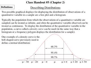
Class Handout #4 (Chapter 1) Definitions Bivariate (Two-Variable) Statistical Inference The one-sample t test about a mean , previously discussed, involves the measurement of only one quantitative variable and provides a good illustration of the concepts behind hypothesis testing in general. However, virtually all hypothesis testing in practice involves at least two variables; a similar comment can be made about confidence intervals. A parametric hypothesis test is designed to focus on one or more parameters in the distribution of a dependent variable often of the continuous type. Such hypothesis tests also generally include an assumption that one or more distributions are normal or that the sample size(s) are sufficiently large to apply some version of the Central Limit Theorem. A nonparametric (or sometimes called distribution-free) hypothesis test is designed to focus on one or more distribution characteristics, not necessarily described by parameters, in the distribution of a dependent variable. Such hypothesis tests do not require any assumption involving either a normal distribution in the data or a dependent variable of the continuous type.
In general, hypothesis testing is often based on a test statistic which involves comparing a numerical measure of the difference between the observed data and what is expected if H0 is true with a numerical measure of some sort of random (error) variation. This general principle remains true for the most part even when the calculations become complex and untenable. The link “Selecting Statistical Analysis” on the web page syllabus leads to a table which displays information about many “basic” statistical analyses in Chapter 1 of the textbook. A dependent (response) variable is one whose changes are being studied, and an independent (explanatory) variable is one which potentially influences changes in a dependent (response) variable.
Pearson Product-Moment Correlation r & Spearman Rank Correlation The Pearson Product-Moment correlation r and the Spearman rank correlation are each a numerical measure of the strength of a linear relationship between two variables X and Y in a data set. If the data are represented by (x1 , y1) (x2 , y2) … (xn , yn) , then we have (x–x)(y–y) , (x–x)2 (y–y)2 r = and we have that is calculated by first replacing the observed values of X by their corresponding ranks s1 , s2 , … , sn ; next replacing the observed values of Y by their corresponding ranks t1 , t2 , … , tn ; and finally calculating the value of r for the rank data represented by (s1 , t1) (s2 , t2) … (sn , tn) . It must always be true that –1 r 1 and –1 1 r = +1 or = +1 corresponds to a perfect positive linear relationship, r = –1 or = –1 corresponds to a perfect negative linear relationship, r = 0 or = 0 corresponds to no linear relationship. Correlations with an absolute value closer to 1 are more indicative of a stronger linear relationship; however, with smaller sample sizes, a given absolute value of correlation is not as significant as with larger sample sizes.
r = +1 or = +1 r or close to +1 r or is positive r or is negative r = –1 or = –1 r or close to –1 r or close to 0 r or close to 0 r or close to 0 r or is negative
It is important to realize that strong correlation between two variables does not imply that changes in one variable will necessarily cause changes in the other. A correlation between two variables which results from each variable being highly correlated to a third is called a spurious correlation. A hypothesis test about the existence of a linear relationship is available with each of the Pearson Product Moment correlation r and the Spearman rank correlation . The H0 states that there is no significant correlation (linear relationship) between variables X and Y. The H1 can be a one-sided or two-sided statement that there is a significant correlation (linear relationship) between variables X and Y. A test statistic based on r assumes that X and Y are each a quantitative-continuous variable with at least one variable having a normal distribution; the corresponding test is considered to be parametric, since the focus is on estimating the correlation between X and Y. A test statistic based on assumes only that X and Y are each either a quantitative variable or a qualitative-ordinal variable; the corresponding test is considered to be nonparametric, since the focus is on rankings instead of actual values. It is not necessary that one variable be considered the dependent variable and the other variable be considered the independent variable. However, when this is the case, we let Y represent the dependent variable and let X represent the independent variable.
When Y represents the dependent variable and X represents the independent variable, then r2 (the square of the Pearson Product-Moment correlation) can be interpreted as the proportion (often converted to a percentage) of variation in the dependent variable Y accounted for by (or explained by) the independent variable X. Go to Exercise #1 on Class Handout #4: 1. Obtain the SPSS output for the example on pages 4 to 6 of the textbook by first selecting options Analyze > Correlate > Bivariate > One-tailed; then, select options Analyze > Correlate > Bivariate > One-tailed > Spearman. Compare the syntax file commands generated by the output with those shown in the textbook. Look at the Analysis: SPSS output section on pages 5 and 6 of the textbook. Finally, create an appropriate graphical display for this data. Tables which give us information about the p-value corresponding to different values of r or with different sample sizes are available, but we shall concentrate on letting SPSS provide us with this information. Results concerning r and stated in the text use conventions/formats popular in the social sciences, but the variations from one discipline to another are generally minor. We shall use a slightly modified format from that in the textbook. For example the results on pages 5 and 6 of the textbook can be written as follows:
1. Obtain the SPSS output for the example on pages 4 to 6 of the textbook by first selecting options Analyze > Correlate > Bivariate > One-tailed; then, select options Analyze > Correlate > Bivariate > One-tailed > Spearman. Compare the syntax file commands generated by the output with those shown in the textbook. Look at the Analysis: SPSS output section on pages 5 and 6 of the textbook. Finally, create an appropriate graphical display for this data. Tables which give us information about the p-value corresponding to different values of r or with different sample sizes are available, but we shall concentrate on letting SPSS provide us with this information. Results concerning r and stated in the text use conventions/formats popular in the social sciences, but the variations from one discipline to another are generally minor. We shall use a slightly modified format from that in the textbook. For example the results on pages 5 and 6 of the textbook can be written as follows: It was found that Pearson’s r = 0.426 (n = 182, p < 0.001) is statistically significant at the 0.05 level (one-tailed). It was found that Spearman’s rho = 0.410 (n = 182, p < 0.001) is statistically significant at the 0.05 level (one-tailed). Thus, the null hypothesis of no correlation is rejected. We conclude that there is a significant negative correlation between levels of self-perception of physical appearance (SelfPerception) and levels of depression (Depression) among college students.
Go to the beginning of Class Handout #4: Independent Samples t-Test Determining whether a relationship exists between a dichotomous variable and a quantitative variable is essentially equivalent to determining whether there is a difference in the distribution of the quantitative variable for each of the two categories of the dichotomous variable. When looking for a difference in the distribution of the quantitative variable for two categories of a dichotomous variable, it is common (but not necessary) to focus on the mean of the distribution. We can let 1and 2 represent the respective means of the quantitative variable for the two categories of the dichotomous variable. In this situation, one can think of the quantitative variable as the dependent variable and the dichotomous variable as the independent variable, that is, we can think of predicting the (mean of the) quantitative variable from the dichotomous variable.
An independent samples t-test, also known as a two-sample t-test, can be used to decide if there is a significant difference in the means. This test is considered to be parametric, since the focus is on estimating the difference in means. The H0 states that the difference between means 1– 2 is 0 (zero), that is, 1= 2 . The H1 can be a one-sided or two-sided statement that there is a significant difference. Two t test statistics are available both based on the assumption that for each of the two categories of the dichotomous variable, the dependent variable is a quantitative-continuous variable having a normal distribution. Each of these test statistics is algebraically similar to the one-sample t test statistic. One of these t statistics, called the pooled t statistic, is also based on the assumption of no difference in the variance of the quantitative variable for the two categories of the dichotomous variable; the other t statistic, called the separate t statistic, is not based on any assumption about the variances of the quantitative variable. (Since both t test statistics give virtually identical results when the population standard deviations are indeed equal, one can always use the separate approach.) A confidence interval for estimating the difference in means can be obtained based either on the assumption of no difference in the variance of the quantitative variable for the two categories of the dichotomous variable, or on no assumption about the variances of the quantitative variable. Go to Exercise #3 on Handout #4:
3. On the west coast of the United States is a chain of restaurants known as McDoogle's. Information about the past year is gathered for a random sample of restaurants in the northern part of the chain, and for a random sample of restaurants in the southern part of the chain; however, for some restaurants, number of customers for the past year was not available. The variables recorded in the data set are a restaurant identification number (ID), the part of the chain in which the restaurant is located (LOCATION), millions of dollars of expenses (EXPEN), millions of dollars of sales (SALES), and millions of customers (CUSTOMER). (Of course, the variable ID is intended only as a label and not intended to be part of any statistical analysis.) The resulting data is as follows: ID LOCATION EXPEN SALES CUSTOMER 01 South 1.0 0.1 3.5 02 North 1.2 1.8 4.4 03 South 2.8 4.0 04 North 1.9 6.1 05 South 0.3 5.3 4.2 06 South 1.5 4.0 0.5 07 South 3.4 7.4 5.1 08 North 1.0 3.6 3.7 09 South 1.6 2.2 10 North 0.9 7.5 3.5
11 North 1.6 4.6 3.1 12 North 1.9 8.0 13 North 0.6 3.3 3.8 14 North 1.0 2.5 3.5 15 South 2.5 2.6 2.4 16 North 1.0 8.1 3.9 17 South 1.9 1.7 1.5 18 North 1.4 6.7 3.5 19 North 0.7 3.8 20 North 1.0 5.2 4.4 21 North 1.3 7.8 22 North 2.4 5.1 4.7 23 North 1.2 7.8 3.7 24 North 1.7 7.7 4.5 25 South 1.4 2.8 3.7 26 North 1.0 4.9 3.5 27 North 1.2 8.0 28 South 2.3 2.0 2.9 29 North 2.2 2.5 4.1 30 North 0.8 5.1 4.2
3.-continued (a) (b) A 0.05 significance level is chosen to see if there is any evidence that the mean number of customers is larger for the northern chain than for the southern chain. State whether a paired t test or a two sample t test should be used and why. Since the data consists of two independent random samples of measurements, a two sample t test should be used. Since it is believed that the standard deviation in number of customers could be quite different for the two chains, it is decided that a separate t test will be used. The data is stored in the SPSS data file chain (created in Exercise #3 of Class Handout #3 Homework). With this data and the appropriate guidelines in the document titled Using SPSS for Windows, use SPSS to do the calculations necessary for the hypothesis test and to create an appropriate graphical display. Then, use the SPSS output to complete the four steps of the hypothesis test by completing the table titled Hypothesis Test About Difference in Mean Number of Customers. Two box plots, one for the for the northern chain and one for the southern chain, are an appropriate graphical display for this hypothesis test.
Hypothesis Test About Difference in Mean Number of Customers Step 1 H0: H1: = Step 2 Step 3 Step 4 N– S = 0 We shall take the approach of always using the separate t test. N – S > 0 0.05 (one sided) nN = xN = sN = nS = xS = sS = 15 3.900 0.4629 t8 = 1.717 8 2.975 1.4859 These statistics can all be obtained from the SPSS output. p-value do not reject H0 from the Student’s t distribution table 0.05 < p < 0.10 t distribution with df = 8 from the SPSS output p = 0.126 / 2 = 0.063 t8; 0.05 = 1.860 OR (p = 0.063) Since t8 = 1.717 and t8; 0.05 = 1.860, we do not have sufficient evidence to reject H0 at the 0.05 level. We conclude that the mean number of customers is not larger for the northern chain than for the southern chain (0.05 < p < 0.10). That is, the difference in mean millions of customers for the northern chain (mean = 3.900, n = 15) and southern chain (mean = 2.975, n = 8) is not statistically significant.
3.-continued Considering the results of the hypothesis test, decide which of the Type I or Type II errors is possible, and describe this error. (c) (d) (e) Since H0 is not rejected, the Type II error is possible, which is concluding that N – S = 0 when actually N – S > 0. Decide whether H0 would have been rejected or would not have been rejected with each of the following significance levels: (i) = 0.01 , (ii) = 0.10 . H0 would not have been rejected with = 0.01 but would have been rejected with = 0.10. Considering the results of the hypothesis test, explain why a confidence interval for the difference between means is not of interest. Since H0 is not rejected, we have no reason to believe that there is a difference between the means; in fact the 95% confidence interval will most likely contain zero the hypothesized difference between means(0). Note that the limits of the confidence interval (displayed on the SPSS output) contain the hypothesized difference between means zero (0).
The two box plots, one for the for the northern chain and one for the southern chain, are an appropriate graphical display for this hypothesis test. It appears that the variation is not the same for both chains. Next class, we will consider a hypothesis test to decide if there is any significant difference in standard deviation, which is what the remainder of this class exercise is concerned with.