Download
1 / 40
400 likes | 578 Views
Error Analysis. Read Ch. 1 & 2 of Packet p. 35, # 2.2, 2.3, 2.5, 2.8 2.12, 2.14, 2.15. Error analysis is the study and evaluation of uncertainty in a measured quantity.

E N D
Error Analysis Read Ch. 1 & 2 of Packet p. 35, # 2.2, 2.3, 2.5, 2.8 2.12, 2.14, 2.15
Error analysis is the study and evaluation of uncertainty in a measured quantity. Science is a discipline ultimately based on measurable quantities and experiences. If it can not be measured, it is not science! It is possible to have a physical theory predict the existence of a yet unmeasured phenomenon, but this phenomenon must be, in principle, measurable. The neutrino is a good example of this: the neutrino was predicted to exist about 40 years before its verification in a laboratory setting. Since the whole structure and application of science is based on measured quantities, it is important to evaluate the limits of measurements due to uncertainty, and evaluate how these uncertainties propagate through calculations. This is the purpose of error analysis.
Inevitability of Uncertainty: Every measured quantity will have a certain amount of uncertainty built into it. Ultimately, these uncertainties are linked to the tolerances and accuracies of the measuring tool and the skill and attentiveness of the individual making the measurement. Every measurement of mass, speed, position, length, time, force, etc, will have some uncertainty attached to it. There are possible exact measurements: There are exactly zero administrators standing in the back of the room, not zero ± three administrators… The above statement does hint at how we represent an uncertainty for a measurement: the ± notation. This notation is used to represent the limit to the confidence of our measurement, or to express the interval where we believe the real measured value lies.
Every measurement involves an estimation: a b 9 cm 10 cm Measurement ‘a’ shown above lies between the markings 9.2 and 9.3 centimeters, so we know that this measured value lies within this range. We can now estimate one more digit between the markings. The estimating gives us the uncertainty. The measured value looks to be about 9.23 cm.
Writing the Measured Value: a b 9 cm 10 cm known for sure estimated value, what are the limits on the estimate?
Judging the Uncertainty: a b 9 cm 10 cm Estimating the uncertainty is a bit of an art, and you have to determine what the limits of your measurement (and measuring process) is. The art of the process is to not underestimate the error, yet not overestimate the error. Underestimating error implies a level of precision not justified in your experiment. Playing safe and overestimating error can yield predictions too broad to be applied. See sections 1.3 – 1.5 of the reading for more on this.
a b ± Notation: 9 cm 10 cm For the diagram above, the markings are wide enough apart that the eye can break the space down into 10 further increments, and your uncertainty would be about ± 1 in that last digit. Thus the measurement would be written as: This can be written shorthand as:
a b ± Notation: 9 cm 10 cm If the markings in the measurement tool were closer together, then subdividing into ten spaces may not be possible. Sometimes you might subdivide into five markings, maybe only two… It is also possible you may not want to subdivide the smallest marking on the measuring tool if you suspect the quality of the construction or possible compromised condition of the measuring tool. ex. metersticks
Rules for Uncertainties: Stating Uncertainties: In an introductory laboratory, experimental uncertainties should usually be rounded to one significant figure. Stating Answers: The last significant figure in any stated answer should usually be of the same order of magnitude (in same decimal position) as the uncertainty. Note: Numbers used in calculations should generally be kept with one more significant figure than is finally justified. This will reduce inaccuracies introduced by rounding the numbers. At the end of the calculation, the final answer should be rounded to remove this extra (and insignificant) figure.
Discrepancy: Discrepancy is defined to be the difference between two measured values of the same quantity. Discrepancy may or may not be significant. Say two students are instructed to determine the length of a given wire indirectly, say from resistivity and resistance measurements. The values the students come up with are: Since these two measurements have uncertainties that overlap, and each students measured value is within the uncertainty range of the other student, this discrepancy is considered insignificant.
Now, lets say the two measurements were as follows: These two measurements are clearly inconsistent, and this discrepancy is significant. Some careful checking of the measuring and calculating process are needed here to find out what went wrong.
Representing Uncertainties: A measurement and its associated uncertainty can be written as follows: or The packet follows the first notation, with the lower case delta. In this form, the uncertainty, by itself, does not say much. For example, an uncertainty of 1 cm for a measurement of the height of a 10 story building would indicate a high precision. An uncertainty of 1 cm for the length of a house fly would indicate a very crude measurement! The uncertainty must be judged in the context of the original measurement.
Fractional (or Relative) Uncertainty: The fractional uncertainty puts the uncertainty in context with the original measurement by writing the uncertainty as a fraction of percent of the original measurement: The uncertainty dx is called the absolute uncertainty. The fractional uncertainty is a dimensionless quantity. This allows measurements of different types or quantities to be compared. For example, the fractional uncertainty for a mass measurement can be compared to the fractional uncertainty of a volume measurement in a density calculation to see which quantity contributes more to the uncertainty of the density.
Propagating Errors through Calculations: If measured quantities are being added or subtracted, the uncertainties add to produce the uncertainty of the sum. Given: The sum and uncertainty become:
Propagating Errors through Calculations: If measured quantities are being multiplied or divided, the fractional uncertainties add to produce the uncertainty of the sum. Given: The product and uncertainty become:
Example #1: The length and width of a rectangle are measured as: Determine the area and perimeter of the rectangle.
Error AnalysisDay #2 Read Ch. 3 & 4 of Packet p. 75, #3.3, 3.4, 3.10; p. 95, #4.1, 4.7
Refinements to Error and Uncertainty Reporting: Consider the sum of some measurements, as shown before: If the measured quantities xi are made independently of one another, and subject only to random errors, the sum of the uncertainties can actually overestimate the uncertainty of the sum.
For example, let’s suppose that the measurement for x1 was underestimated (i.e. larger than reported) and the measurement for x2 was overestimated (i.e. smaller than reported), but both were within the estimated uncertainty range, ± dxi. When these quantities are added together, the overestimation of one compensates the underestimation of the other, tending to reduce the effect of the error. The straight sum of uncertainties will overestimate the uncertainty for this case. This possibility (one overestimate, one underestimate) has a 50% possibility of occurring, so 50% of the time the straight sum of uncertainties will overestimate the uncertainty of the sum.
When dealing with independent measurements, a better system of dealing with uncertainties involves using Normal or Gaussian distributions. The details will be left to Mr. Rod’s sadistics (er, statistics) class. The general outcome is this: If quantities are measured independently and subject to random errors, a better estimate for the uncertainty of a sum is found by adding the individual uncertainties in quadrature: The quadrature result is a better estimate of the uncertainty, and the straight sum is greatest possible uncertainty.
When computing a product, just add the percent uncertainties in quadrature as well.
Example #1: The length and width of a rectangle are measured as: Determine the area and perimeter of the rectangle.
General Functions and Error Propagation. A more general expression for the product formula can be given as follows: Suppose F is a function of several variables in the form: Here, A is a constant. a,b,c are constants for the powers of x,y,z. The uncertainty for F is given as:
An even more general version is given on p.73 of the packet: F is a general function of x,y,z. The uncertainty for function F is given as:
Example #2: Two charged pith balls of equal mass and equal charge are suspended from strings from a common center, as shown below. Determine the charge on the balls. Analysis shows that the charge is given as: The given values are:
Random Errors: For several measurements made in the same way, the uncertainties can be broken into two main categories: random and systematic. Experimental uncertainties that can be revealed by repeating the measurements are called random errors. An example of systematic error would be parallax issues arising on a meter stick. Systematic uncertainties cannot be revealed with repeated measurements with the same measuring tools. An example would be using a stopwatch that runs slow (or fast). This would be something that could not be revealed unless another timing mechanism was available.
Standard Deviation: Suppose some quantity has been measured several times, such as the density of aluminum objects, and the systematic errors have been reduced to a negligible level. What will represent the best estimate for the several measurements? The best estimate is given as the average of the values:
The next step would be to estimate the average uncertainty of the measurements. The average uncertainty of the measurements is usually called the standard deviation, and is calculated as follows: Consider the difference between the individual data points and the average, the best estimated value. This difference is called the deviation of measurement xi from the average. This is defined as: If the deviations are small, then the measurements are considered precise. Note that deviations may be negative. As an exercise, try to show that the average of the deviations is zero.
In the Physics – B class, a tool used to evaluate data using the concept of deviation was the average absolute deviation. This is easy enough to calculate, but it does tend to overestimate the differences (and the error). The standard deviation takes care of this by adding the terms effectively in quadrature, and gives a better estimate of the error. Unfortunately, there are two definitions of standard deviation.
The population standard deviation is defined as the square root of the average of the square of the deviations: The alternative definition is the sample standard deviation: The population version tends to underestimate the uncertainty by a small amount, so the sample version divides N – 1 to correct this.
The sample standard deviation is the preferred tool for determining the closeness of several measured values. Based on the results of the Normal or Gaussian distributions, the sample standard deviation may be used as a way to estimate the uncertainty in the best estimated value. This would be written as: In this form, we can say that any individual measurement (from the same equipment) has a 70% probability of being within this range of the averaged measurement.
Standard Deviation of the Mean The average of the individual measurements represents the best estimated value of the group of measurements. The sample standard deviation characterizes the average uncertainty of the group of measurements. It turns out though, the average best estimate represents a very reliable representation of the data, more reliable than any one individual measurement considered separately. From the theory of Gaussian distributions, a better estimate of the uncertainty associated with the average is the sample standard deviation divided by the square root of the number of measurements: Standard Deviation of the Mean or Standard Error or Standard Error of the Mean
Thus the best estimate and uncertainty is written in the form: Just be sure to label what each type of uncertainty is that you report, so that the readers may judge for themselves which uncertainty to hold as more significant.
Example #3: Hans – Jürgen has measured the density of several copper objects, and has come up with the following values. Determine the average and the standard deviation of the mean for his data.
Just use your calculator to find the value of the sample standard deviation. The standard deviation function on your calculator is just this function shown above. 70% of the data points should be within this distance of the averaged value.