Download
1 / 106
1.06k likes | 1.27k Views
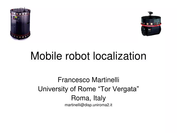
Mobile robot localization. Francesco Martinelli University of Rome “Tor Vergata” Roma, Italy martinelli@disp.uniroma2.it. Objective :. Determination of the pose (= position + orientation) of a mobile robot in a known environment in order to succesfully perform a given task. Summary :.

E N D
Mobile robot localization Francesco Martinelli University of Rome “Tor Vergata” Roma, Italy martinelli@disp.uniroma2.it
Objective: Determination of the pose (= position + orientation) of a mobile robot in a known environment in order to succesfully perform a given task
Summary: • Robot localization taxonomy (4-5) • Robot localization as an estimation problem: the Bayes filter (6-17) • Observability issue (18-23) • Robot description (24) • Motion model: the differential drive (25-34) • Measurement model: rangefinder or landmarks (35-39) • Robot localization algorithms (40-42): • Gaussian filters: EKF, UKF (43-60) • Non parametric filters: HF, PF (61-77) • Examples (78-104) • Conclusions (105) • References (106) • Video
Robot Localization Taxonomy: • Position tracking • Global localization • Kidnapped problem Increasing degree of difficulty • Other classifications include: • type of environment (static or dynamic; completely or partially known) • active or passive localization • single or multi robot localization.
Robot Localization Taxonomy: • Position tracking • Global localization • Kidnapped problem Increasing degree of difficulty • Other classifications include: • type of environment (static or dynamic; completely or partially known) • active or passive localization • single or multi robot localization.
Localization as an estimation problem The robot must infer its pose from available data Data (noisy): • Motion information: • Proprioceptive sensors (e.g. encoders, accelerometers, etc.) • Environment Measurements • Exteroceptive sensors (e.g. laser, sonar, IR, GPS, camera, RFID, etc.) A filtering approach is required to fuse all information
Localization as an estimation problem Notation y q Robot pose x Robot poses from time 0 to time t Robot exteroceptive measurements from time 1 to time t Motion commands (or proprioceptive measurements) from time 0 to time t
Localization as an estimation problem Notation Belief of the robot at time t: probability density function (pdf) describing the information the robot has regarding its pose at time t, based on all available data (exteroceptive measurements and motion commands): Prior belief of the robot at time t: pdf before acquiring the last measurement zt:
Localization as an estimation problem Notation The robot motion model is the pdf of the robot pose at time t+1 given the robot pose and the motion action at time t. It takes into account the noise characterizing the proprioceptive sensors: The measurement model describes the probability of observing at time t a given measurement zt when the robot pose is xr,t. It takes into account the noise characterizing the exteroceptive sensors:
Localization as an estimation problem The Bayes Filter Prediction Motion model Robot pose space Based on the total probability theorem: (discrete case) where Bi, i=1,2,... is a partition of W. In the continuous case:
Localization as an estimation problem The Bayes Filter - Prediction Illustration of the prediction step in an ideal case Assume a robot moving along a unidimensional space, i.e. xr = x, and assume an ideal motion model: x
Localization as an estimation problem The Bayes Filter - Prediction Illustration of the prediction step in a realistic case Still a unidimensional space but consider a more realistic motion model: where the noise x
Localization as an estimation problem The Bayes Filter Correction or Measurement Update Normalizing factor Measurement model Based on the Bayes Rule: i.e. also: Taking: We have:
Localization as an estimation problem The Bayes Filter - Correction Illustration of the correction step in an ideal case Assume a robot moving along a unidimensional space, i.e. xr = x, and measuring the distance to a landmark placed in the origin. Under an ideal measurement model: zt = z = x x
Localization as an estimation problem The Bayes Filter - Correction Illustration of the correction step in a realistic case Still a unidimensional space, still the robot is measuring the distance to a landmark placed in the origin. Under a realistic measurement model: where the noise zt = z = x+n x
Localization as an estimation problem The Bayes Filter It is a recursive algorithm. At time t, given the belief at time t-1 belt-1(xr), the last motion control ut-1 and the last measurement zt, determine the new belief belt(xr) as follows: For all xr do the following: Motion model Measurement model
Localization as an estimation problem The Bayes Filter - Observations • The Bayes filter is not a practical algorithm • Gaussian Filters: Extended Kalman Filter (EKF), • Unscented Kalman Filter (UKF), • Extended Information Filter (EIF) • Non Parametric Filters: Histogram Filter (HF), • Particle Filter (PF) • Important to check if we have enough information to localize the robot • (observability issue). • Sometimes the observability can be evaluated through the • observability rank condition (see Hermann&Krener, TAC 1977)
Observability issue The robot may have not enough sensors to determine its pose, even if assuming perfect (i.e. without noise) measurements. The robot is equipped with encoder readings and can measure the distance r to a landmark located in the origin. y ri = range measurement at time ti dij = distance covered (and measured) by the robot in time interval [ti,tj] t3 r3 x d23 r2 Dq2 = robot turn at time t2 (known from odometry) r1 Dq2 d12 t2 t1 In the figure we represent two different robot paths agreeing with measurements. The robot poseis not completely observable: there is a radial symmetry around the origin
Case the robot measures (with noise) the distance from two landmarks (in addition to the odometry). The robot pose is not completely observable. Observability issue True path Path reconstructed through the EKF (position tracking) The noise makes the estimated pose jump to the specular path.
Observability issue In the nonlinear case, the observability depends on the particular control input considered. Hence, the possibility of localizing a mobile robot may depend on the particular motion executedwhich in any case affects the localization performance Active Localization The robot is equipped with odometry and measures the angle j (a non symmetric landmark is located in the origin). y dij = distance covered (and measured) by the robot in time interval [ti,tj] t3 d23 d12 t2 Under this motion (radial) the distance of the robot from the origin (hence x and y) cannot be determined but only the orientation q = j t1 j x
Observability issue A different kind of motion would make the pose observable (active localization): The robot is equipped with odometry and measures the angle j (a non symmetric landmark is located in the origin). y j1 j2 dij = distance covered (and measured) by the robot in time interval [ti,tj] j3 t2 t1 d23 d12 t3 Under this motion all the pose of the robot can be determined x
Observability issue Often localization is performed under a generic motion(passive localization): the robot tries to localize itself while performing its mission (once a satisfactory pose estimation has been reached) or under a random motion away from obstacles (at the beginning, when the pose is still completely unknown).
Observability issue This is because usually mobile robots are equipped with several sensors: they can often localize themselves even if not moving (e.g. if measuring the distance to at least 3 non collinear landmarks). Nevertheless... problems may arise with symmetrical environments (the robot has odometry + rangefinder, e.g. sonar or laser). A proper robot motion may disambiguate in some cases the pose estimation.
Robot description • Motion model (proprioceptive sensors) From Thrun Burgard Fox, Probabilistic Robotics, MIT Press 2006 • Measurement model (exteroceptive sensors)
Motion model Motion model (proprioceptive sensors) Assume: • xr,t robot pose at time t • ut control input (i.e. motion command) at time t Which is the pose at time t+1? Usually, ut is obtained through proprioceptive sensors (e.g. encoders, gyroscopes, etc) Odometry motion model Due to sensor noise, xr,t+1 is available only through a probability density function. From Thrun Burgard Fox, Probabilistic Robotics, MIT Press 2006
Different wheeldiameters (systematic source of noise) Carpet (casual source of noise) Ideal case Bump (casual source of noise) Motion model Possible sources of noise and many more (e.g. distance between the wheels) … From Thrun Burgard Fox, Probabilistic Robotics, MIT Press 2006
Motion model Accumulation of the pose estimation error under the robot motion (only proprioceptive measurements) From Thrun Burgard Fox, Probabilistic Robotics, MIT Press 2006
Motion model Discretized unicycle model: Robot shift in time interval [t,t+1] Robot rotation in time interval [t,t+1] y dqt xr,t drt xr,t+1 x
Motion model Discretized unicycle model: the differential drive case Minibot
Motion model Differential drive uR,t = distance covered by the Right wheel in [t,t+1] uL,t = distance covered by the Left wheel in [t,t+1] d = distance between the wheels y d If the sampling time is small enough: dqt xr,t+1 drt xr,t dqt x D
Motion model Differential drive There is a bijective relation between (dr, dq) and (uR, uL): Mismatch between real (uR,t, uL,t) and measured (uR,te, uL,te) distances covered by the wheels of the robot. The encoder readings are related to the real distances covered by the two wheels as follows: (casual source of noise)
Motion model Differential drive Estimation (red points) of the path covered by a differential drive robot. Blue = real position in each step. Starting point
Motion model Differential drive Given: • xr,t = [x,y,q]^T robot pose at time t, • encoder reading ut = [uRe, uLe]^T (i.e.result of the control input) relative to • the interval [t, t+1], we want to estimate the probability that the robot pose at time t+1 will be a given xr,t+1= [x’,y’,q’]^T (under the differential drive model considered), i.e.:
Motion model We proceed as follows: Differential drive Actual robot displacement if we want to arrive at [x’,y’,q’]^T from [x,y,q]^T: Corresponding distances covered by the two wheels, while the actual encoder readings are (uRe, uLe): The probability of arriving in [x’,y’,q’]^T from [x,y,q]^T is the probability of reading (uRe, uLe) when the actual wheel shifts are (uR, uL)
Measurement model (exteroceptive sensors) Assume: • xr,t robot pose at time t Which is the reading zt of a sensor at time t? Due to sensor noise, zt is available only through a probability density function.
Measurement model (exteroceptive sensors) Two typical settings are considered: Range Finder (e.g. laser or sonar readings). The environment is known and is represented by line segments (e.g. the walls). The robot senses the distance from them at some given directions. Landmark measurements. The environment is characterized by features (artificial or natural landmarks), whose position is known and whose identity can be known (e.g. RFID tags) or must be estimated (data association problem). The robot measures the distance and/or the bearing to these fixed points.
Measurement model: the Range Finder case Each measurement zi,t is a range measurement tipically based on the time of flight of the beam (e.g. of a sonar or a laser) generated by sensor i and reflected by an obstacle Measurement given by beam i Distance of sensor i from the reflecting obstacle (ideal reading of the sensor)
Measurement model: the Range Finder case Given: • xr,t = [x,y,q]^T robot pose at time t, we want to estimate the probability that the measurement of sensor i (with orientationqiwith respect to the robot motion direction) at time t is a given zt. yp P • First compute the distance • hi(xrt) between sensor i and • the reflecting point P • (this is possible given the robot pose • since the environment is assumed • known) qi q y xp x • Then:
Measurement model: landmark measurements Let xr,t = [x,y,q]^T be the robot pose at time t Assuming known the identities (and the position) of the landmarks, for each landmark Li = (xi,yi) there is a measurement Li yi where ri,t ji,t q y and xi x
Robot Localization Algorithms The application of the Bayes filter is referred to as Markov Localization: For all xr do the following: Motion model Measurement model … in the case of Global Localization
Robot Localization Algorithms Example of Markov Localization (here xr = x) z0: door detected From Thrun Burgard Fox, Probabilistic Robotics, MIT Press 2006 u0: the robot moves z1: door detected again u1: the robot moves again L
Robot Localization Algorithms • The Bayes filter is not a practical algorithm • Gaussian Filters: Extended Kalman Filter (EKF), • Unscented Kalman Filter (UKF), • Extended Information Filter (EIF) • Non Parametric Filters: Histogram Filter (HF), • Particle Filter (PF)
Robot Localization Algorithms Gaussian filters (EKF, UKF) • Tractable implementations of the Bayes Filter obtained by means of a • Gaussian approximation of the pdf • Unimodal approximations completely defined through mean m and covariance P • OK for Position Tracking or in the global case if measurements allow • to restrict the estimation to a small region (e.g. RFID) • The robot detects a corner and sees only • free corridors Bimodal pdf. • A bimodal pdf is not well approximated • through a Gaussian density • Multi-Hypothesis Gaussian (also in the case of unknown data association)
Robot Localization Algorithms Extended Kalman Filter (EKF) Gaussian In the linear-gaussian case, all steps of the Bayes filter result in gaussian pdf the Kalman Filter (KF) is optimal for these systems. EKF: extension of KF to non linear systems (no more optimal) Linear-gaussian system: Process noise Measurement noise Assume:
Robot Localization Algorithms Prediction step (Bayes filter) Gaussian - EKF ... is the convolution of two Gaussian distributions still Gaussian! The Kalman Filter results in the update of mean m and covariance P: where: Prediction Step KF
Robot Localization Algorithms Gaussian - EKF Correction step (Bayes Filter) ... is the product of two Gaussian distributions still Gaussian! The Kalman Filter results in the update of mean m and covariance P: where: Kalman Gain Correction Step KF innovation
Robot Localization Algorithms Extension to non linear systems (EKF) Gaussian - EKF Non linear - Gaussian system: Process noise Measurement noise Assume:
Robot Localization Algorithms Prediction Step KF Gaussian - EKF Prediction Step EKF Correction Step KF Correction Step EKF
Robot Localization Algorithms Application to the localization problem: Gaussian - EKF
Robot Localization Algorithms Unscented Kalman Filter (UKF) Gaussian Specific for non linear systems: avoids jacobians and derives the pdf of a random variable transformed through a non linear function through the transformation of a set of Sigma Points. Same numerical complexity of EKF. Generally more performant, but still not optimal! Let a scalar gaussian random variable. Let be a non linear function. Clearly y is not gaussian. If using Gaussian filters, y is approximated through a Gaussian random variable, i.e.: