Download
1 / 68
690 likes | 939 Views
Numerical Methods for Sparse Systems. Ananth Grama Computer Sciences, Purdue University ayg@cs.purdue.edu http://www.cs.purdue.edu/people/ayg. Review of Linear Algebra. A square matrix can be viewed as a graph. Rows (or columns) form vertices. Entries in the matrix correspond to edges.

E N D
Numerical Methods for Sparse Systems Ananth Grama Computer Sciences, Purdue University ayg@cs.purdue.edu http://www.cs.purdue.edu/people/ayg
Review of Linear Algebra • A square matrix can be viewed as a graph. • Rows (or columns) form vertices. • Entries in the matrix correspond to edges. • A dense matrix corresponds to a completely connected graph. • A sparse matrix with bounded non-zeros/row corresponds to a graph of bounded degree. • This is a very convenient view of a matrix from the point of view of parallel operations on a matrix.
Graph of a Matrix The graph of a symmetric matrix is undirected.
Graph of a Matrix Graph of a non-symmetric matrix is directed.
Origins of Sparse Matrices Discretization of a Laplacian operator using centered differences to a 2D grid results in a pentadiagonal matrix. Similarly, matrices from finite element discretizations preserve topological correspondence between domain and the graph of the matrix.
Matrix-Vector Product Communication is only along edges in the graph of the matrix
Other operations: LU Factorization Elimination of rows corresponds to generating a clique of neighbors.
Parallelizing Matrix-Vector Products • If the degree of each node in the graph of the matrix is bounded, the computation per node in the graph is bounded since each edge corresponds to one multiply-add. • Load can be balanced by assigning equal number of nodes in the graph to each processor.
Parallelizing Matrix-Vector Product • The question of which nodes should go to which processor is determined by minimizing the communication volume. • Since each edge in the graph corresponds to one incoming data item, minimizing edge cut across partitions also minimizes volume of communication.
Parallelizing Matrix-Vector Products: Algorithm • Start with the graph of the matrix. • Partition the graph into p equal parts such that the number of edges going across partitions is minimized. • Assign each partition to one processor. • At each processor, gather incoming vector data from each edge. • Compute local dot products.
Partitioning Graphs for Minimum Edge Cuts • Recursive orthogonal coordinate bisection. • Slide a partitioner along an axis for equipartition. • Recursive spectral bisection. • Use second eigenvector (Fiedler vector) of the Laplacian of the graph to order/partition graph. This process can be expensive. • Multilevel methods. • Coarsen the graph, partition coarse graph using, say, spectral methods and project partitions back, refining the projection at each step.
Multilevel Graph Partitioning Packages such as Metis [Karypis, Kumar, Gupta] and Chaco [Hendrickson] are capable of partitioning graphs with millions of nodes within seconds.
Performance of Matrix-Vector Products • The computation associated with a partition is equal to the number of nodes (volume) in the partition. • The communication associated is equal to the surface area of the partition. • Using good partitioners, the volume to surface ratio can be maximized, yielding good computation to communication ratio.
Implications for serial performance • Graph reordering is useful for serial performance as well. • By ordering the nodes in a proximity preserving order, we can maximize reuse of the vector (note that the matrix elements are only reused once, but vector elements are used as many times as the degree of corresponding node). • Using spectral ordering of nodes, performance improvements of over 50% have been shown.
Superlinearity Effects • Often, people show superlinear speedups in sparse matrix-vector products. • This is a result of extra cache available to the parallel formulation. • Such effects are sometimes symptomatic of a poor serial implementation. • These effects can (and should) be minimized by using optimal serial implementations.
Summary of Parallel Matvecs Ordered/partitioned matrix
Computing Dot-Products in Parallel • This is the other key primitive needed for implementing the most basic iterative solvers. • Dot products can be implemented by computing local dot products followed by a global reduction.
Other Vector Operations • Vector addition: Since the nodes are partitioned across processors and vector elements sit on nodes, vector addition is completely local with no communication. • Norm Computation: This requires a reduction operation (similar to dot product). • Multiplication by a scalar: Completely local operation with no communication.
Basic Iterative Methods • The Jacobi Method Ax = b (L + D + U)x = b x = D-1(b - (L + U)x) x(n+1) = D-1(b - (L + U)x(n)) • Each iteration requires: • one matrix-vector product: (L + U)x(n), • one vector addition: (b - (L + U)x(n)), • one diagonal scaling: D-1(b - (L + U)x(n)) • one norm computation: | x(n+1) - x(n)| • Each of these can be easily computed in parallel using operations that we have discussed.
Gauss-Seidel Algorithm Ax = b (L + D + U)x = b x = D-1(b - (L + U)x) x(n+1) = D-1(b - Ux(n)- Lx(n+1)) The idea is to use the most recent components of the solution vector to compute next iterate.
Successive Overrelaxation (SOR) • Computes the weighted average of the nth and (n+1)st iterates. Xn+1 = (1-w) xn + w D-1(b - Ux(n)- Lx(n+1)) • Convergence is shown for 0 < w < 2. • Parallel processing issues are identical to Gauss Seidel Iterations. • Color the nodes and split each iteration into two - one for nodes of each color.
Conjugate Gradients • One of the most common methods for symmetric positive definite systems. • In each iteration, solution x is updated as x = x + ap • Here, p is the search direction and a is the distance the solution travels along the search direction. • Minimization of error leads to a specific choice of a and p. • The approximate solution is mathematically encompassed by the set {r0, Ar0, A2r0, …, Anr0}.
Conjugate Gradients 1 vector addition, 1 norm, 1 scalar product 1 mat-vec, 1 dot product 1 scalar product, 1 vector addition 1 vector addition Total: One mat-vec, two inner products, three vector adds
Conjugate Gradients: Parallel Implementation • Matrix-vector product can be parallelized by partitioning the matrix and vector. • Two inner products can be parallelized using a reduce operation. • All other operations are local and do not require any communication.
GMRES-Parallel Implementation • In addition to parallel matrix vector products, GMRES involves an Arnoldi process. • Arnoldi process builds an orthonormal basis for the Krylov subspace. • As soon as a new vector is added, it is orthogonalized w.r.t. previous vectors. • Modified Gram-Schmidt is preferred for numerical stability. However, this requires considerable communication. • Householder transforms (block Househonder factorization in parallel) can also be used. However, it can be expensive. • Block orthogonalization can be used but this slows convergence.
Preconditioning for Accelerating Convergence • While trying to solve Ax = b, if A is the identity matrix, any iterative solver would converge in a single iteration. • In fact, if A is “close” to identity, iterative methods take fewer iterations to converge. • We can therefore solve: M-1Ax = M-1b where M is a matrix that is close to A but is easy to invert.
Preconditioning Techniques • Explicitly construct M-1 and multiply it by A and b before applying an iterative method. The problem with this method is that the inverse of a sparse matrix can be dense so we must somehow limit the “fill” in M-1. • Alternately, since the key operation inside a solver is to apply a matrix to a vector (Ax), to apply (M-1A)x, we can use: M-1Ax = b, Mb = Ax, Mb = c That is, we can solve a simpler system similar to A in each preconditioning step.
Preconditioning Techniques • Diagonal Scaling. M = diag(A), • M-1 can be applied by dividing the vector by corresponding diagonal entries. • Where there is a mat-vec (Ax) in the iterative method, compute Ax = c, and divide each element of c by the corresponding diagonal entry. • In a parallel solver with a row based partitioning of the matrix, this does not introduce any additional communication.
Preconditioning Techniques • Diagonal scaling attempts to localize the problem to the single node with no boundary conditions. • A generalization of this problem divides the graph into partitions and inverts these partitions. • The way the boundary conditions are enforced determine the specific solution technique.
Preconditioning: Schwarz Type Schemes No forcing terms - convergence properties are not good.
Preconditioning: Additive Schwarz Allow overlap between processor domains. These overlaps provide boundary conditions for individual domains. If all processors work on their sub-domains concurrently, the method is called an Additive Schwarz method. There is excellent parallelism since after the matvec and communication of overlapping values of right hand side, all computation is local.
Preconditioning: Multiplicative Schwarz • Also relies on overlapping domains. • However, sub-domain solves are performed one after the other, using most recent values from the previous solve. • This ordering in Multiplicative Schwarz serializes the preconditioner! • Parallelism can be regained by coloring the subdomains red and black and performing the computation in red phase followed by black phase (similar to Gauss Seidel).
Multigrid Methods • Start from the original problem. A few relaxation steps are carried out to smooth high frequency errors (smoothing). • Residual errors are injected to a coarse grid (injection). • This process is repeated to the coarsest grid and the problem is explicitly solved here. • The correction is interpolated back by successive smoothing and projection.
Multigrid: V-Cycle Algorithm • Perform relaxation on AhUh = fh on fine grid until error is smooth. • Compute residual, rh = fh - AhUh and transfer to the coarse grid r2h = I2hh rh. • Solve the coarse-grid residual equation to obtain the error: A2h e2h = r2h. • Interpolate the error to the fine grid and correct the fine-grid solution: uh=uh +Ih2h e2h
Multigrid Methods Relaxation is typically done using a lightweight scheme (Jacobi/GS). These can be performed in parallel on coarse meshes as well. The issue of granularity becomes important for the coarsest level solve.
Parallel Multigrid • In addition to the nodes within the partition, maintain a additional layer of “ghost” values that belong to the neighboring processor. • This ghost layer can be increased (a la Schwarz) to further reduce the number of iterations.
Incomplete Factorization • Consider again: • To solve individual sub-domains, each processor computes L and U factors of local sub-blocks. Since this is not a true LU decomposition of the matrix, it is one instance of an Incomplete LU factorization.
Incomplete Factorization • Computing full L and U decomposition of the matrix can be more expensive (see second part of this tutorial). • Therefore a number of approximations are used to reduce associated computation and storage. • These center around heuristics for dropping values in the L and U factors.
Incomplete Factorization • There are two classes of heuristics used for dropping values: • Drop values based on their magnitude (thresholded ILU factorization). • Drop values based on level of fill - ILU(n). Fill introduced by original matrix element is level 1 fill, fill introduced by level 1 fill is level 2 fill, and so on. • It is easy to see that ILU(0) allows no fill. • Parallel formulations of these follow from parallel factorization techniques discussed in the second part of this tutorial.
Approximate Inverse Methods • These methods attempt to construct an approximate inverse of A while limiting fill. A M ~ I • There are mainly two approaches to constructing a sparse approximate inverse: • Factored sparse approximate inverse. • Construct the approximate inverse as: min ||AM - I||F • The Frobenius norm is particularly useful since
Approximate Inverse Methods • Solving the minimization equation leads to the following n independent least squares problems: • A number of heuristics are used to bound the number of non-zeros in each column of the approximate inverse. • The bound follows from the decay in values in the sparse approximate inverse.
Approximate Inverse Methods Decay in the inverse of a Laplacian