Download
1 / 16
160 likes | 274 Views
Beyond δN-formalism for a single scalar field. Resceu, University of Tokyo Yuichi Takamizu 27th Sep@COSMO/CosPA2010 Collaborator: Shinji Mukohyama (IPMU,U of Tokyo), Misao Sasaki & Yoshiharu Tanaka (YITP,Kyoto U) Ref : JCAP06 019 (2010) & JCAP01 013 (2009). ◆ Introduction.

E N D
Beyond δN-formalismfor a single scalarfield Resceu, University of Tokyo Yuichi Takamizu 27th Sep@COSMO/CosPA2010 Collaborator: Shinji Mukohyama (IPMU,U of Tokyo), Misao Sasaki & Yoshiharu Tanaka (YITP,Kyoto U) Ref: JCAP06 019 (2010)& JCAP01 013 (2009)
◆Introduction ●Non-Gaussianity from inflation Slow-roll ? Single field ? Canonical kinetic ? • Standard single slow-roll scalar • Many models predicting Large Non-Gaussianity • ( Multi-fields, DBIinflation & Curvaton) WMAP 7-year PLANK2009- • Non-Gaussianity will be one of powerful tool to discriminate many possible inflationary modelswith the future precision observations
●Nonlinear perturbations on superhorizon scales • Spatial gradient approach : Salopek & Bond (90) • Spatial derivatives are small compared to time derivative • Expand Einstein eqs in terms of small parameter ε, and can solve them for nonlinear perturbations iteratively (Starobinsky 85, Sasaki & Stewart 96 Sasaki & Tanaka 98) ◆δNformalism (Separated universe ) Curvature perturbation = Fluctuations of the local e-folding number ◇Powerful tool for the estimation of NG
◆Temporary violating of slow-roll condition • e.g.Double inflation, False vacuum inflation (Multi-field inflation always shows) For Single inflaton-field (this talk) ◆δNformalism • Ignore the decaying mode of curvature perturbation ◆Beyond δNformalism • Decaying modes cannot be neglected in this case • Enhancementof curvature perturbation in the linear theory [Seto et al (01), Leach et al (01)]
◆Example ●Starobinsky’s model(92): • There is a stage at which slow-roll conditions are violated • Linear theory • The in the expansion ●Leach, Sasaki, Wands & Liddle (01) Violating of Slow-Roll Decaying mode Decaying mode Growing mode • Enhancement of curvature perturbation near
m ●Nonlinear perturbations on superhorizon scales up to Next-leading order in the expansion =Full nonlinear n 1 2 …… ∞ 0 ・・δN 2 ・・Beyond δN ……. 2nd order perturb n-th order perturb Linear theory ∞
◆Beyond δN-formalism for single scalar-field YT, S.Mukohyama, M.Sasaki & Y.Tanaka JCAP(2010) Simple result ! • Nonlinear variable (including δN) • Nonlinear Source term ●Nonlinear theory in Ricci scalar ofspatial metric ●Linear theory
◆Application of Beyond δN-formalism ●To Bispectrum for Starobinsky model :Ratio of the slope of the potential Even for ●Temporary violation of slow-rolling leads to particular behavior (e.g. sharp spikes) of the power & bispectrum Localized feature models • These features may be one of powerful tool to discriminate many inflationary models with the future precision observations
◆Beyond δN-formalism System : • Single scalar field with general potential & kinetic term including K- inflation & DBI etc ●ADMdecomposition & Gradient expansion Small parameter: ◆Backgroundis the flat FLRWuniverse Basic assumption: • Absence of any decaying at leading order • Can be justified in most inflationary model with
Solve the Einstein equation after ADM decomposition in Uniform Hubble +Time-orthogonal slicing ●General solution YT& Mukohyama, JCAP 01(2009) valid up to ●Curvature perturbation Spatial metric Constant (δN ) • Variation of Pressure (speed of soundetc) • Scalar decaying mode
◆Nonlinear curvature perturbation YT, Mukohyama, Sasaki & Tanaka , JCAP06 (2010) Complete gauge fixing Focus on onlyScalar-type mode ●What is a suitable definition of NL curvature perturbation ? Perturbation of e-folding Cf)δN-formalism ? Need this term in this formula in
Decaying mode Growing mode YT, Mukohyama, Sasaki & Tanaka (10) ◆Second-order differential equation Scalar decaying mode Constant (δN ) Some integrals satisfies Ricci scalar of 0th spatial metric ●Natural extension of well-known linear version
◆Matching conditions Our nonlinear sol (Grad.Exp) Standard perturbative sol In order to determine the initial cond. General formulation:Valid in the case that the value & its deri.of the N-th order perturb. solutions are given ◆Matched Nonlinear sol to linear sol Approximate Linear sol around horizon crossing @ ● Final result Enhancement in Linear theory δN Nonlinear effect
◆Application to Starobinsky model • There is a stage at which slow-roll conditions are violated ●In Fourier space, calculate Bispectrum ◆ Equilateral ◆ Shape of bispectrum equil Local
◆Applications of our formula (Temporary violating of slow-roll condition) Calculate the integrals; • Non-Gaussianity in this formula matched to DBI inflation • Apply to varying sound velocity • Trispectrumof the feature models • Extension to nonlinear Gravitational wave • Extension to the models of Multi-scalar field (with Naruko,in progress) • (naturally gives temporary violating of slow-roll cond)
◆Summary • We develop a theory of nonlinear cosmological perturbations on superhorizon scales for a scalar field with a general potential & kinetic terms • We employ the ADM formalism and the spatial gradient expansion approach to obtain general solutions valid up through second-order • We formulate a general method to match n-th order perturbative solution • Can applied to Non-Gaussianity in temporary violating of slow-rolling • Beyond δN-formalism: Two nonlinear effects • ①Nonlinear variable : including δN (full nonlinear) • ②Nonlinear source term : Simple2nd order diff equation • Calculate the bispectrumfor the Starobinsky model