Download
1 / 38
380 likes | 499 Views
The sensitivity of fire-behavior and smoke-dispersion indices to the diagnosed mixed-layer depth Joseph J. Charney U.S. Forest Service, Northern Research Station, Lansing, MI and Daniel Keyser

E N D
The sensitivity of fire-behavior and smoke-dispersion indices to the diagnosed mixed-layer depth Joseph J. Charney U.S. Forest Service, Northern Research Station, Lansing, MI and Daniel Keyser Department of Atmospheric and Environmental Sciences, University at Albany, State University of New York, Albany, NY
Organization • Background • Objective • Double Trouble State Park (DTSP) Wildfire Event • WRF Model Configuration • Indices and Diagnostics • Results • Conclusions
Background The goal of this project is to diagnose the spatial and temporal variability of meteorological quantities in the planetary boundary layer that can affect fire behavior and smoke dispersion. Meteorologists and fire and smoke managers are currently debating the manner in which the mixed-layer depth is, and should be, diagnosed.
Background While fire-behavior and smoke-dispersion indices are sensitive to diagnosed mixed-layer depth (MLD), the potential for sensitivities in the indices to affect fire- and smoke-management decisions is not well-understood. A quantitative assessment of these sensitivities can help enable fire and smoke managers to anticipate whether the implementation of a given MLD diagnostic could affect their ability to fulfill burn program requirements.
Objective • We will assess the sensitivity of a fire-behavior index and a smoke-dispersion index to three MLD diagnostics using mesoscale model simulations of the 2 June 2002 DTSP wildfire event. • Indices: • fire-behavior index: downdraft convective available potential energy (DCAPE) • smoke-dispersion index: Ventilation Index (VI) • MLD diagnostics: • surface-based buoyancy • potential temperature(z) = potential temperature(sfc) • potential temperature(z) = potential temperature(z/2) • z = height above ground level
DTSP Wildfire Event • Occurred on 2 June 2002 in east-central NJ • Abandoned campfire grew into major wildfire by 1800 UTC • Burned 1,300 acres • Forced closure of the Garden State Parkway • Damaged or destroyed 36 homes and outbuildings • Directly threatened over 200 homes • Forced evacuation of 500 homes • Caused ~$400,000 in property damage • References: • Charney, J. J., and D. Keyser, 2010: Mesoscale model simulation of the meteorological conditions during the 2 June 2002 Double Trouble State Park wildfire. Int. J. Wildland Fire, 19, 427–448. • Kaplan, M. L., C. Huang, Y. L. Lin, and J. J. Charney, 2008: The development of extremely dry surface air due to vertical exchanges under the exit region of a jet streak. Meteor. Atmos. Phys., 102, 63–85.
DTSP Wildfire Event "Based on the available observational evidence, we hypothesize that the documented surface drying and wind variability result from the downward transport of dry, high-momentum air from the middle troposphere occurring in conjunction with a deepening mixed layer." "The simulation lends additional evidence to support a linkage between the surface-based relative humidity minimum and a reservoir of dry air aloft, and the hypothesis that dry, high-momentum air aloft is transported to the surface as the mixed layer deepens during the late morning and early afternoon of 2 June." (Charney and Keyser 2010)
WRF Model Configuration • WRF version 3.4 • 4 km nested grid • 51 sigma levels, with 21 levels in the lowest 2000 m • NARR data for initial and boundary conditions • Noah land-surface model • RRTM radiation scheme • YSU PBL scheme
Indices and Diagnostics DCAPE • DCAPE is the maximum kinetic energy that can be realized by the parcel, which is proportional to the area indicated in brown on the diagram (Emanuel 1994, pp. 172–173). • DCAPE calculation: • Choose a starting level for the parcel • Saturate the parcel • Bring the parcel to the surface while maintaining saturation • For the starting level: • Potter (2005) proposes 3000 m • We choose the top of the MLD
Indices and Diagnostics DCAPE DCAPE was originally formulated to estimate the maximum strength of evaporatively cooled downdrafts beneath a convective cloud (Emanuel 1994, p. 172-173). It has been suggested that DCAPE could be applied to wildland fires (Potter 2005). We hypothesize that in the case of a mixed layer produced by dry convection, large DCAPE may correlate well with low surface relative humidity when the mixed-layer is deep and the top of the mixed layer is dry.
Indices and Diagnostics Ventilation Index (VI) Definition: the MLD multiplied by the “transport wind speed” The transport wind speed can be interpreted in several different ways: • mixed-layer average wind speed • surface wind speed (usually 10 m) • 40 m wind speed For the purposes of this study, the mixed-layer averaged wind speed will be used.
Indices and Diagnostics Ventilation Index (VI) From Hardy et al. (2001)
Indices and Diagnostics MLD Diagnostics 1) MLD1 is diagnosed by determining the height to which near-surface eddies can rise freely. The parcel exchange potential energy (PEPE) as proposed by Potter (2002) is employed. The lowest height at which PEPE is zero is identified as the top of the surface-based mixed layer.
Indices and Diagnostics MLD Diagnostics LeMoneand coauthors, in their presentation at the 12th Annual WRF Users’ Workshop (20–24 June 2011, National Center for Atmospheric Research, Boulder, CO), proposed a number of mixed-layer diagnostics for use with mesoscale model output.
Indices and Diagnostics MLD Diagnostics 2) MLD2 is diagnosed by finding the highest level above the ground where the potential temperature equals the surface potential temperature. Ɵ mixed-layer height height potential temperature
Indices and Diagnostics MLD Diagnostics 3) MLD3 is diagnosed by finding the highest level above the ground where the potential temperature equals the potential temperature at one half that height above the ground. mixed-layer height height z z/2 potential temperature
Results Time series of MLD1, MLD2, and MLD3 (m)
Results Skew T diagram showing the pressure at the top of the mixed layer for MLD1, MLD2, and MLD3 at 1300 UTC
Results Skew T diagram showing the pressure at the top of the mixed layer for MLD1, MLD2, and MLD3 at 1700 UTC
Results Skew T diagram showing the pressure at the top of the mixed layer for MLD1, MLD2, and MLD3 at 2100 UTC
Results Time series of DCAPE (J/kg) using MLD1, MLD2, and MLD3
Results Time series of VI (m2/s) using MLD1, MLD2, and MLD3
Results Correlations of DCAPE using MLD1 with MLD1 and with surface and mixed-layer average moisture variables from 1200 UTC to 2100 UTC 2 June 2002
Results Correlations of DCAPE using MLD2 with MLD2 and with surface and mixed-layer average moisture variables from 1200 UTC to 2100 UTC 2 June 2002
Results Correlations of DCAPE using MLD3 with MLD3 and with surface and mixed-layer average moisture variables from 1200 UTC to 2100 UTC 2 June 2002
Results Time–height cross section of RH with time series of MLD1, DCAPE using MLD1, and surface RH MLD1
Results Time–height cross section of RH with time series of MLD2, DCAPE using MLD2, and surface RH MLD2
Results Time–height cross section of RH with time series of MLD3, DCAPE using MLD3, and surface RH MLD3
Results Time–height cross section of TDD with time series of MLD1, DCAPE using MLD1, and surface TDD MLD1
Results Time–height cross section of TDD with time series of MLD2, DCAPE using MLD2, and surface TDD MLD2
Results Time–height cross section of TDD with time series of MLD3, DCAPE using MLD3, and surface TDD MLD3
Results Time–height cross section of RH with time series of MLD1, DCAPE using MLD1, and mixed-layer average RH using MLD1 MLD1
Results Time–height cross section of RH with time series of MLD2, DCAPE using MLD2, and mixed-layer average RH using MLD2 MLD2
Results Time–height cross section of RH with time series of MLD3, DCAPE using MLD3, and mixed-layer average RH using MLD3 MLD3
Results Time–height cross section of TDD with time series of MLD1, DCAPE using MLD1, and mixed-layer average TDD using MLD1 MLD1
Results Time–height cross section of TDD with time series of MLD2, DCAPE using MLD2, and mixed-layer average TDD using MLD2 MLD2
Results Time–height cross section of TDD with time series of MLD3, DCAPE using MLD3, and mixed-layer average TDD using MLD3 MLD3
Conclusions MLD diagnostics produce differences ~100-200 m in a simulation of the DTSP wildfire. Differences in MLD diagnostics contribute to DCAPE values that differ by ~20-25%. Differences in MLD diagnostics produce VI values that differ by 4000-6000 m2/s. The diurnal variation in DCAPE is shown to correlate with MLD and with meteorological variables that diagnose low-level moisture.