Download
1 / 22
220 likes | 332 Views
GEOG 3404 Economic Geography. LECTURE 4: Transportation, Cost-Distance and Industrial Location Central Place Theory. Dr. Zachary Klaas Department of Geography and Environmental Studies Carleton University. Transportation costs: Or, “the death of distance has been greatly exaggerated.”.

E N D
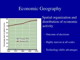
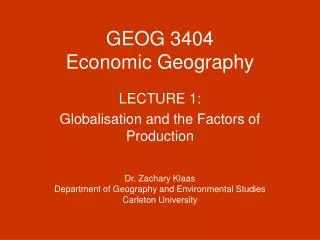
GEOG 3404Economic Geography LECTURE 4: Transportation, Cost-Distance and Industrial Location Central Place Theory Dr. Zachary Klaas Department of Geography and Environmental Studies Carleton University
Transportation costs: Or, “the death of distance has been greatly exaggerated.” • In today’s lecture, we will deal with the effect of transportation costs on economies at a local, regional and world scale. The continuing existence of real costs associated with transporting goods from one location to another (or, perhaps, transporting people from one location to another where they are to provide services) is one potential argument against the “death of distance” hypothesis in economic geography. So long as transporting things involve a cost, distance matters in the world economy. • This will lead us to formulate general conceptions of cost-distance measurement – in other words, measurement of distance in terms of the costs that occur when the distance is traversed.
We will address cost-distance as a geographic concept from a number of vantage points. First we will consider the issue of industrial location. Where a firm locates is in part a decision about how far the firm will have to transport its products. Another important concern is mode of transport. Historical changes in kinds of transportation have affected economic developments drastically. • Then we will address the issue by noting how the development of transport networks contribute to the ease (or lack thereof) of transporting a firm’s products. We will consider the extent to which the connectivity of a matrix affects the efficiency of a regional economy, as well as the issue of whether transport networks have adequate infrastructure support as well as functioning capacity and a general lack of congestion. • Finally, we will consider how distance has a primary role in the creation of a central place system – a spatial arrangement of urban areas across a landscape according to the interrelating requirements of producers and consumers of goods and services.
Transportation and cost-distance • In our previous work for this class, we have seen that the cost of transporting freight was a key element of the von Thünen model. The variables k (distance) and f (freight costs) are both modeled in von Thünen’s equation, and they are multiplied together in that equation with E (units produced). Assuming that each of these values is over zero, any rise in E, f or k raises costs. To put this another way, the Efk term of the von Thünen equation is a cost-distance measure based on an assessment specifically of the costs of transportation. • All geography is concerned, at some level, with distance, and similarly, all economic geography is, at some level, concerned with cost-distance. The effect that traversing distance has on economic interactions is central to what the economic geographer’s occupations.
Industrial location: The conscious attempt to minimise transport costs • If transporting goods to a marketplace create real costs, and one wishes to minimise these costs in order to make profits rather than pay out to cover these costs with the proceeds of one’s sales, then there are a number of industrial location strategies which recommend themselves. • If the production process for the goods intended to be sold in the marketplace acts to lower the costs of transport, then it is logical to locate a production facility (i.e., a factory) as near to the locations of the natural resources used to make the product as possible. • If the production process for the goods intended to be sold in the market place acts to raise the costs of transport, then it is logical to locate a production facility (i.e., a factory) as near to the marketplace location as possible.
Alfred Weber’s model for industrial location • The German economic geographer Alfred Weber (brother of the somewhat more well-known sociologist Max Weber) developed a deductive model to specify where the best sites for the location of production facilities (i.e., factories) would be, based on transportation costs. • Essentially, Weber’s main variable for the assessment of the cost-distance associated with production was weight. If a product weighed more, it was generally costlier to transport. Thus, if it could be determined what the weight differential would be between unprocessed raw materials from nature and fully processed products, it would be easier to determine where to locate the factory. • If production lowers the weight of the final product, Weber concluded, the factory should be by the natural resource site. If it raises the weight, the factory should be by the marketplace.
Of course, it is fairly typical for products to contain within them more than one kind of natural resource input. A given product might be fashioned from many natural resources, which could come from any number of natural resource site locations. This requires some consideration of midway points in the model. • This being the case, the factory might have to be located close to a number of different natural resource sites. Weber’s model is premised on the concept of a locational triangle between (at least) two natural resource sites and one marketplace. • If the processing of each natural resource input reduces weight for the product, then the proper location of the production facilities would likely be at the midpoint between the resource sites on the side of the triangle the farthest from the marketplace. • However, if processing any input adds weight to the final product, then this would pull the proper location of the production facilities towards the marketplace. Midway point locations
More about Weber’s theory • If there are numerous natural resource sites involved in making a product, of course, then more than just one triangle will have to be used to locate the proper place for the production facilities. Weber used the triangles to geometrically construct lines called isotims which could identify the lowest-cost locations for production facilities. • Weber’s theory was based on certain assumptions which in reality do not always hold true. One such assumption had to do with the spatial location patterns of labourers working at the production facilities. It is possible, of course, that a factory could draw in mobile labourers from elsewhere, but it might also be that a labouring population (especially those who perform particularly skilled labour) might convince factory owners to locate their facilities closer to them.
Still more about Weber’s theory • Weber also did not consider agglomeration (the location of similar businesses in the same geographic location) as part of this model. Locating production facilities more remotely from supporting businesses might be the source of costs not measured by the model. • Weber’s model is pretty much exclusively consumed with understanding line-haul costs, or costs that increase with distance. But there are also terminal costs, which are costs that are unrelated to distance, to consider, and terminal costs might be different at different locations for the production facilities. • Weber’s model also seems to presume that one is unconcerned with the specific mode of transport being employed – weight affects all transportation, he seems to reason. But weight does not affect each mode of transport equally. A firm owner might prefer a weighty cargo, but on a jet, to a light cargo but on horse drawn carts. The jet is suited to handle heavier cargo.
Mode of transport • One clear historical development affecting cost-distance is the physical mode of transport actually involved in getting the product from natural resource site to production facility to marketplace. The experience of distance has greatly diminished due to dramatic improvements in mode of transport. • Peter Dicken’s book for this course shows, on page 81, a quite interesting graphic for how mode of transport “shrinks” the world by allowing the same distance to be traversed in less time. • Until 1840, the top speed of travel was around 16 kph; until 1930, ships traveled around 58 kph and trains around 104 kph on average; by the 1950s, propeller aircraft travelled at roughly 480-640 kph, and by the 1960s, jet aircraft travelled at roughly 800-960 kph.
Mode of transport and related costs • What mode of transport one is using to transport goods has a strong bearing on both terminal costs (which are not affected by distance – analogous to the notion of fixed costs in economics generally) and on line-haul costs (which are affected by distance – analogous to the notion of variable costs in economics generally): • Line haul costs: • It takes more trips of smaller conveyances (trucks, airplanes) than it would take of larger conveyances (trains, ships) to move the same amount of goods. • Terminal costs: • Capital investment for supporting facilities for certain conveyances (ports for ships, airports for airplanes) may be higher than for other conveyances (truck yards for trucks, train stations for trains).
More about mode of transport and related costs • There can also be the phenomenon of curvilinear line-haul costs. This is more or less the distance version of an economy of scale (which is what one has when a firm is able to increase its efficiency the larger it becomes). In the case of curvilinear line-haul costs, one is able to increase one’s efficiency at transporting goods the longer the distance one has to go. • A curvilinear line-haul cost reflects larger increases in cost-distance to a certain distance, but then smaller increases in cost-distance after a certain “breaking point”. • With large-scale modes of transport, it is often little worth the trip to transport over a small distance, but increasingly worthwhile over larger distances.
Transport networks • Thus far, we have spoken of transportation, but we have not addressed the networks over which transportation occurs (such as roads / railways, but also such as systems of interaction between stations / ports / airports.) • The construction of physical transport networks is an important infrastructure cost to be considered. One can have very efficient modes of transport but not be able to utilise them due to the poor state of this necessary infrastructural support. • Physical transport networks also have the capability of being congested. In other words, they can be used to such an extent that it is not possible to accommodate traffic at a level sufficient for present purposes. When congestion occurs, one has to contemplate either reining in use of the network, or expansion of the network.
Types of transport networks • The objective for the construction or maintenance of transport networks is to create a least-cost path, or a route along the network that minimises some kind of costs. • There are numerous strategies for doing this, depending on the kind of cost one is trying to minimise: • Branching networks connect locations by means of paths that meet at midpoints between the locations; this kind of network minimises construction costs. • Circuit networks connect locations by means of paths that directly connect all the locations; this kind of network minimises user costs. • “Hub and spoke” networks connect locations to one location where some kind of central facility is sited; this kind of network minimises costs by centralising production at a key site. It is also a kind of network which is most prominent in the organisation of the air travel and air delivery industries, which route airplanes through hub destinations to save money.
Route travel models: Paul Revere’s Ride and the Travelling Salesman • There are also least-cost path models involving how one addresses having to visit every location in a network while incurring the least possible costs. • If you have to visit every location, but once at the last location, you don’t have to go back to the one you started from, the Paul Revere’s Ride model is the one which identifies the order in which you will have to visit the locations in the network. (Paul Revere had to visit all the cities to warn of the impending British attack, but once all cities were visited, he did not have to return home to warn everyone there again.) • If you have to visit every location, but once at the last location, you do have to go back to the one you started from, the Traveling Salesman model is the one which identifies the order in which you will have to visit the locations in the network. (A traveling salesman has to visit all his sales locations, but then go home again, and ultimately repeat the process at a later time.)
“Virtual” networks • Nowadays, we have increasing experience of “virtual” networks – that is, networks where distance seems not to play a role. On our computers, for example, we can often download something from Europe, Japan, Australia or New Zealand with the same relative ease as from a server physically right next door to us. • In material terms, really, “virtual” networks aren’t wholly virtual. Telecommunications can make it seem that way, but only after cables are laid across swaths of the globe (as well as under the sea) traversing long physical distances. • There are important geographically-based cost-distances to consider here, though. Areas with less infrastructural support for telecommunications networks may be harder to reach via virtual networks – hence in terms of virtual cost-distance, Asia, Africa and Latin America may be “further away”. Note the graphic on page 91 of Dicken.
Congestion • Congestion is an issue in both physical and virtual networks. When networks become overloaded by users, one must either rein in the use of the network or expand the network. • If you build it, they will come. Sometimes an unintended effect of expansion of a network is that network use is increased at a large scale, due to the availability of network support for that scale of use. Transportation planners have observed this phenomenon and actually advocated failing to respond to demands for more roads on the basis that it will rein in an already destructively large over-reliance on automobile transportation. Building the road would not, by this view, reduce congestion, which would expand to meet the size of the new network. • The same for the internet – does widening network bandwidths simply make it possible for download sizes to get unmanageably large?
Connectivity • Connectivity is another issue in networks of importance to economic geographers. The connectivity of a network is reflected by its beta index – the ratio of paths connecting the network to the number of nodes, or locations connected by the network. • Presumably, a network with a high number of paths per node offers numerous routes to a destination, avoiding overloaded routes, and generally offers direct routes between the nodes, avoiding circuitous or unnecessarily long routes. • Mere connectivity is not always the whole story. It is possible that some paths in a network involve more cost-distance to travel than others. Another measure of connectivity is therefore what is called an index of accessibility, which weights the beta index according to the cost-distance involved in using the paths.
Central place theory • Moving on to a slightly different but related theme in economic geography – how is the establishment of a business firm related to the size or proximity of a population settlement in space? • The German economic geographer Walter Christaller observed that the size and spacing of settlements could be predicted across a given space, in what can be called the central place pattern. The central place pattern allows an area to be serviced economically by firms providing higher-order goods and services (those requiring larger population bases) as well as those providing lower-order goods and services (those requiring only small population bases). • The central place pattern his model predicted for southern Germany was quite close to the pattern of settlement that actually existed there at the time.
Central place theory has two functioning parts involved with its predictive model – THRESHOLD and RANGE: • The threshold of a given product is the number of people in a population which must be present or nearby in order to purchase that product. • High-order products require a high threshold – for example, a major-league sports team requires a high threshold to pay for the massive overhead of maintaining a stadium, paying all the team’s players, and organising the games played. This requires the support of thousands of people, or the team will not be able to get off the ground financially. • Low-order products, by contrast, only require a low threshold – for example, a hot dog vendor only needs to sell hot dogs to around twenty or thirty people daily, which is nowhere near the thousands the sports team requires. • The range of a given product is the distance members of a population are willing to travel in order to purchase a product. • High-order products require a high range – for example, a neurosurgeon can count on people traveling a long distance for the services the neurosurgery office provides, as these kinds of services are necessary and not available everywhere. • Low-order products, by contrast, only benefit from a low range – for example, people are not willing to travel too far to get to a service station which sells gasoline for their cars. The obvious expectation is that gas stations should be located close to the car owners.
Threshold and range: the basis of “higher” and “lower” orders of centres • Urban centres which have high populations are places which can support firms requiring high thresholds. Thus, products requiring a high population base are more likely to locate in larger cities, which themselves provide this high population base, even without respect to other places in the central place pattern. • Urban centres which are near high populations are places which can support firms with high ranges. Thus, if the population base for a product is not found in a particular urban centre, the range of the product can assist in finding the necessary population base in nearby areas in the larger central place pattern.
Spacing of higher-order and lower-order centres • Christaller’s central place pattern is an arrangement of heartlands and hinterlands. Heartlands are population centres – the big cities which provide population bases for the highest-order goods. Hinterlands are nearby regions to the heartland locations, where there is less population but a population capable of travel to the larger centres for their economic needs. • The population constant K in Christaller’s model is used as the mathematical basis for the spacing out of settlements of different sizes according to the requirements of the model. This constant reflects the size of difference between levels of population in cities as well as the amount of distance between settlements between cities in the pattern.