Download
1 / 56
560 likes | 562 Views
This lecture discusses the performance of storage devices and the application of queueing theory in operating systems and systems programming. Topics covered include memory-mapped display controllers, transferring data to/from controllers, I/O device notification, device drivers, and basic performance concepts.

E N D
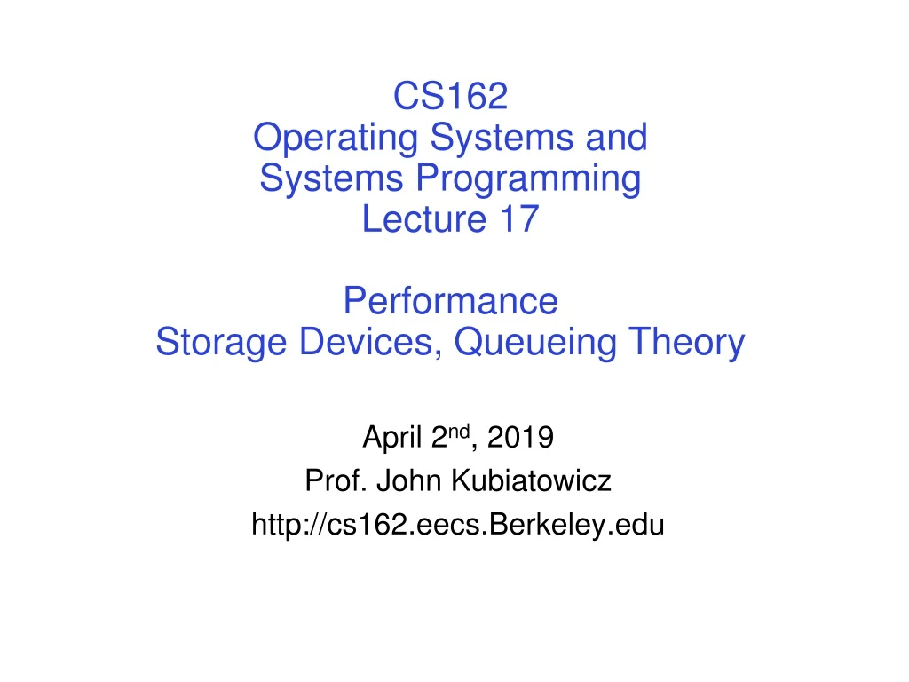
CS162Operating Systems andSystems ProgrammingLecture 17PerformanceStorage Devices, Queueing Theory April 2nd, 2019 Prof. John Kubiatowicz http://cs162.eecs.Berkeley.edu
0x80020000 Graphics Command Queue 0x80010000 Display Memory 0x8000F000 Command 0x0007F004 Status 0x0007F000 Physical Address Space Recall: Memory-Mapped Display Controller • Memory-Mapped: • Hardware maps control registers and display memory into physical address space • Addresses set by HW jumpers or at boot time • Simply writing to display memory (also called the “frame buffer”) changes image on screen • Addr: 0x8000F000 — 0x8000FFFF • Writing graphics description to cmd queue • Say enter a set of triangles describing some scene • Addr: 0x80010000 — 0x8001FFFF • Writing to the command register may cause on-board graphics hardware to do something • Say render the above scene • Addr: 0x0007F004 • Can protect with address translation
Transferring Data To/From Controller • Programmed I/O: • Each byte transferred via processor in/out or load/store • Pro: Simple hardware, easy to program • Con: Consumes processor cycles proportional to data size • Direct Memory Access: • Give controller access to memory bus • Ask it to transfer data blocks to/from memory directly • Sample interaction with DMA controller(from OSC book): 1 2 3
Transferring Data To/From Controller • Programmed I/O: • Each byte transferred via processor in/out or load/store • Pro: Simple hardware, easy to program • Con: Consumes processor cycles proportional to data size • Direct Memory Access: • Give controller access to memory bus • Ask it to transfer data blocks to/from memory directly • Sample interaction with DMA controller(from OSC book): 4 5 6
I/O Device Notifying the OS • The OS needs to know when: • The I/O device has completed an operation • The I/O operation has encountered an error • I/O Interrupt: • Device generates an interrupt whenever it needs service • Pro: handles unpredictable events well • Con: interrupts relatively high overhead • Polling: • OS periodically checks a device-specific status register • I/O device puts completion information in status register • Pro: low overhead • Con: may waste many cycles on polling if infrequent or unpredictable I/O operations • Actual devices combine both polling and interrupts • For instance – High-bandwidth network adapter: • Interrupt for first incoming packet • Poll for following packets until hardware queues are empty
Device Drivers • Device Driver: Device-specific code in the kernel that interacts directly with the device hardware • Supports a standard, internal interface • Same kernel I/O system can interact easily with different device drivers • Special device-specific configuration supported with the ioctl() system call • Device Drivers typically divided into two pieces: • Top half: accessed in call path from system calls • implements a set of standard, cross-device calls like open(),close(),read(),write(),ioctl(),strategy() • This is the kernel’s interface to the device driver • Top half will start I/O to device, may put thread to sleep until finished • Bottom half: run as interrupt routine • Gets input or transfers next block of output • May wake sleeping threads if I/O now complete
Life Cycle of An I/O Request User Program Kernel I/O Subsystem Device Driver Top Half Device Driver Bottom Half Device Hardware
Basic Performance Concepts • Response Time or Latency: Time to perform an operation(s) • Bandwidth or Throughput: Rate at which operations are performed (op/s) • Files: MB/s, Networks: Mb/s, Arithmetic: GFLOP/s • Start up or “Overhead”: time to initiate an operation • Most I/O operations are roughly linear in bbytes • Latency(b) = Overhead + b/TransferCapacity
Example (Fast Network) • Consider a 1 Gb/s link (B = 125 MB/s) • With a startup cost S = 1 ms • Latency(b) = S + b/B • Bandwidth = b/(S + b/B) = B*b/(B*S + b) = B/(B*S/b + 1)
Example (Fast Network) • Consider a 1 Gb/s link (B = 125 MB/s) • With a startup cost S = 1 ms • Half-power Bandwidth B/(B*S/b + 1) = B/2 • Half-power point occurs at b=S*B= 125,000 bytes
Example: at 10 ms startup (like Disk) • Half-power b = 1,250,000 bytes!
What Determines Peak BW for I/O ? • Bus Speed • PCI-X: 1064 MB/s = 133 MHz x 64 bit (per lane) • ULTRA WIDE SCSI: 40 MB/s • Serial Attached SCSI & Serial ATA & IEEE 1394 (firewire): 1.6 Gb/s full duplex (200 MB/s) • USB 3.0 – 5 Gb/s • Thunderbolt 3 – 40 Gb/s • Device Transfer Bandwidth • Rotational speed of disk • Write / Read rate of NAND flash • Signaling rate of network link • Whatever is the bottleneck in the path…
Storage Devices • Magnetic disks • Storage that rarely becomes corrupted • Large capacity at low cost • Block level random access (except for SMR – later!) • Slow performance for random access • Better performance for sequential access • Flash memory • Storage that rarely becomes corrupted • Capacity at intermediate cost (5-20x disk) • Block level random access • Good performance for reads; worse for random writes • Erasure requirement in large blocks • Wear patterns issue
Read/Write Head Side View IBM/Hitachi Microdrive Western Digital Drive http://www.storagereview.com/guide/ Hard Disk Drives (HDDs) • IBM Personal Computer/AT (1986) • 30 MB hard disk - $500 • 30-40ms seek time • 0.7-1 MB/s (est.)
The Amazing Magnetic Disk • Unit of Transfer: Sector • Ring of sectors form a track • Stack of tracks form a cylinder • Heads position on cylinders • Disk Tracks ~ 1µm (micron) wide • Wavelength of light is ~ 0.5µm • Resolution of human eye: 50µm • 100K tracks on a typical 2.5” disk • Separated by unused guard regions • Reduces likelihood neighboring tracks are corrupted during writes (still a small non-zero chance)
The Amazing Magnetic Disk • Track length varies across disk • Outside: More sectors per track, higher bandwidth • Disk is organized into regions of tracks with same # of sectors/track • Only outer half of radius is used • Most of the disk area in the outer regions of the disk • Disks so big that some companies (like Google) reportedly only use part of disk for active data • Rest is archival data
Shingled Magnetic Recording (SMR) • Overlapping tracks yields greater density, capacity • Restrictions on writing, complex DSP for reading • Examples: Seagate (8TB), Hitachi (10TB)
Head Cylinder Review: Magnetic Disks • Cylinders: all the tracks under the head at a given point on all surface • Read/write data is a three-stage process: • Seek time: position the head/arm over the proper track • Rotational latency: wait for desired sector to rotate under r/w head • Transfer time: transfer a block of bits (sector) under r/w head Track Sector Platter Seek time = 4-8ms One rotation = 1-2ms (3600-7200 RPM)
Head Cylinder Software Queue (Device Driver) Hardware Controller Media Time (Seek+Rot+Xfer) Request Result Review: Magnetic Disks • Cylinders: all the tracks under the head at a given point on all surface • Read/write data is a three-stage process: • Seek time: position the head/arm over the proper track • Rotational latency: wait for desired sector to rotate under r/w head • Transfer time: transfer a block of bits (sector) under r/w head Track Sector Platter Disk Latency = Queueing Time + Controller time + Seek Time + Rotation Time + Xfer Time
Disk Performance Example • Assumptions: • Ignoring queuing and controller times for now • Avg seek time of 5ms, • 7200RPM Time for rotation: 60000 (ms/min) / 7200(rev/min) ~= 8ms • Transfer rate of 50MByte/s, block size of 4Kbyte 4096 bytes/50×106 (bytes/s) = 81.92 × 10⁻⁶ sec 0.082 ms for 1 sector • Read block from random place on disk: • Seek (5ms) + Rot. Delay (4ms) + Transfer (0.082ms) = 9.082ms • Approx 9ms to fetch/put data: 4096 bytes/9.082×10-3 s 451KB/s • Read block from random place in same cylinder: • Rot. Delay (4ms) + Transfer (0.082ms) = 4.082ms • Approx4ms to fetch/put data: 4096 bytes/4.082×10-3 s 1.03MB/s • Read next block on same track: • Transfer (0.082ms): 4096 bytes/0.082×10-3 s 50MB/sec • Key to using disk effectively (especially for file systems) is to minimize seek and rotational delays
(Lots of) Intelligence in the Controller • Sectors contain sophisticated error correcting codes • Disk head magnet has a field wider than track • Hide corruptions due to neighboring track writes • Sector sparing • Remap bad sectors transparently to spare sectors on the same surface • Slip sparing • Remap all sectors (when there is a bad sector) to preserve sequential behavior • Track skewing • Sector numbers offset from one track to the next, to allow for disk head movement for sequential ops • …
Example of Current HDDs • Seagate Exos X14 (2018) • 14 TB hard disk • 8 platters, 16 heads • Helium filled: reduce friction and power • 4.16ms average seek time • 4096 byte physical sectors • 7200 RPMs • 6 Gbps SATA /12Gbps SAS interface • 261MB/s MAX transfer rate • Cache size: 256MB • Price: $615 (< $0.05/GB) • IBM Personal Computer/AT (1986) • 30 MB hard disk • 30-40ms seek time • 0.7-1 MB/s (est.) • Price: $500 ($17K/GB, 340,000x more expensive !!)
Solid State Disks (SSDs) • 1995 – Replace rotating magnetic media with non-volatile memory (battery backed DRAM) • 2009 – Use NAND Multi-Level Cell (2 or 3-bit/cell) flash memory • Sector (4 KB page) addressable, but stores 4-64 “pages” per memory block • Trapped electrons distinguish between 1 and 0 • No moving parts (no rotate/seek motors) • Eliminates seek and rotational delay (0.1-0.2ms access time) • Very low power and lightweight • Limited “write cycles” • Rapid advances in capacity and cost ever since!
SSD Architecture – Reads Read 4 KB Page: ~25 usec • No seek or rotational latency • Transfer time: transfer a 4KB page • SATA: 300-600MB/s => ~4 x10³ b / 400 x 106 bps => 10 us • Latency = Queuing Time + Controller time + Xfer Time • Highest Bandwidth: Sequential OR Random reads NAND NAND NAND NAND Host Buffer Manager (software Queue) Flash Memory Controller NAND NAND NAND NAND SATA NAND NAND NAND NAND NAND NAND NAND NAND NAND NAND NAND NAND NAND NAND NAND NAND NAND NAND NAND NAND NAND NAND NAND NAND DRAM
SSD Architecture – Writes • Writing data is complex! (~200μs – 1.7ms ) • Can only write empty pages in a block • Erasing a block takes ~1.5ms • Controller maintains pool of empty blocks by coalescing used pages (read, erase, write), also reserves some % of capacity • Rule of thumb: writes 10x reads, erasure 10x writes https://en.wikipedia.org/wiki/Solid-state_drive
Some “Current” 3.5in SSDs • Seagate Nytro SSD: 15TB (2017) • Dual 12Gb/s interface • Seq reads 860MB/s • Seq writes 920MB/s • Random Reads (IOPS): 102K • Random Writes (IOPS): 15K • Price (Amazon): $6325 ($0.41/GB) • Nimbus SSD: 100TB (2019) • Dual port: 12Gb/s interface • Seqreads/writes: 500MB/s • Random Read Ops (IOPS): 100K • Unlimited writes for 5 years! • Price: ~ $50K? ($0.50/GB)
HDD vs SSD Comparison SSD prices drop much faster than HDD
Amusing calculation: Is a full Kindle heavier than an empty one? • Actually, “Yes”, but not by much • Flash works by trapping electrons: • So, erased state lower energy than written state • Assuming that: • Kindle has 4GB flash • ½ of all bits in full Kindle are in high-energy state • High-energy state about 10-15 joules higher • Then: Full Kindle is 1 attogram (10-18gram) heavier (Using E = mc2) • Of course, this is less than most sensitive scale can measure (it can measure 10-9 grams) • Of course, this weight difference overwhelmed by battery discharge, weight from getting warm, …. • Source: John Kubiatowicz(New York Times, Oct 24, 2011)
SSD Summary • Pros (vs. hard disk drives): • Low latency, high throughput (eliminate seek/rotational delay) • No moving parts: • Very light weight, low power, silent, very shock insensitive • Read at memory speeds (limited by controller and I/O bus) • Cons • Small storage (0.1-0.5x disk), expensive (3-20x disk) • Hybrid alternative: combine small SSD with large HDD
SSD Summary • Pros (vs. hard disk drives): • Low latency, high throughput (eliminate seek/rotational delay) • No moving parts: • Very light weight, low power, silent, very shock insensitive • Read at memory speeds (limited by controller and I/O bus) • Cons • Small storage (0.1-0.5x disk), expensive (3-20x disk) • Hybrid alternative: combine small SSD with large HDD • Asymmetric block write performance: read pg/erase/write pg • Controller garbage collection (GC) algorithms have major effect on performance • Limited drive lifetime • 1-10K writes/page for MLC NAND • Avg failure rate is 6 years, life expectancy is 9–11 years • These are changing rapidly! No longer true!
Response Time (ms) 300 Controller User Thread I/O device 200 Queue [OS Paths] 100 Response Time = Queue + I/O device service time 0 100% 0% Throughput (Utilization) (% total BW) I/O Performance • Performance of I/O subsystem • Metrics: Response Time, Throughput • Effective BW per op = transfer size / response time • EffBW(n) = n / (S + n/B) = B / (1 + SB/n ) # of ops time per op Fixed overhead
Response Time (ms) 300 Controller User Thread I/O device 200 Queue [OS Paths] 100 Response Time = Queue + I/O device service time 0 100% 0% Throughput (Utilization) (% total BW) I/O Performance • Performance of I/O subsystem • Metrics: Response Time, Throughput • Effective BW per op = transfer size / response time • EffBW(n) = n / (S + n/B) = B / (1 + SB/n ) • Contributing factors to latency: • Software paths (can be loosely modeled by a queue) • Hardware controller • I/O device service time • Queuing behavior: • Can lead to big increases of latency as utilization increases • Solutions?
A Simple Deterministic World • Assume requests arrive at regular intervals, take a fixed time to process, with plenty of time between … • Service rate (μ = 1/TS) - operations per second • Arrival rate: (λ = 1/TA) - requests per second • Utilization: U = λ/μ , where λ< μ • Average rate is the complete story Queue Server arrivals departures TQ TS TA TA TA TS Tq
A Ideal Linear World • What does the queue wait time look like? • Grows unbounded at a rate ~ (Ts/TA) till request rate subsides 1 Saturation 1 Delivered Throughput Delivered Throughput Empty Queue Unbounded 0 1 0 1 Offered Load (TS/TA) Offered Load (TS/TA) Queue delay Queue delay time time
A Bursty World • Requests arrive in a burst, must queue up till served • Same average arrival time, but almost all of the requests experience large queue delays • Even though average utilization is low Queue Server arrivals departures TQ TS Arrivals Q depth Server
So how do we model the burstiness of arrival? • Elegant mathematical framework if you start with exponential distribution • Probability density function of a continuous random variable with a mean of 1/λ • f(x) = λe-λx • “Memoryless” Likelihood of an event occurring is independent of how long we’ve been waiting mean arrival interval (1/λ) Lots of short arrival intervals (i.e., high instantaneous rate) Few long gaps (i.e., low instantaneous rate) x (λ)
Mean (m) Distribution of service times mean Memoryless Background: General Use of Random Distributions • Server spends variable time (T) with customers • Mean (Average) m = p(T)T • Variance (stddev2) 2 = p(T)(T-m)2 = p(T)T2-m2 • Squared coefficient of variance: C = 2/m2Aggregate description of the distribution • Important values of C: • No variance or deterministic C=0 • “Memoryless” or exponential C=1 • Past tells nothing about future • Poisson process – purely or completely random process • Many complex systems (or aggregates)are well described as memoryless • Disk response times C 1.5 (majority seeks < average)
Controller Disk Queue Departures Arrivals Queuing System Introduction to Queuing Theory • What about queuing time?? • Let’s apply some queuing theory • Queuing Theory applies to long term, steady state behavior Arrival rate = Departure rate • Arrivals characterized by some probabilistic distribution • Departures characterized by some probabilistic distribution
Little’s Law • In any stablesystem • Average arrival rate = Average departure rate • The average number of jobs/tasks in the system (N) is equal to arrival time / throughput (λ) times the response time (L) • N (jobs) = λ(jobs/s) x L (s) • Regardless of structure, bursts of requests, variation in service • Instantaneous variations, but it washes out in the average • Overall, requests match departures N arrivals departures λ L
Example λ = 1 L= 5 L = 5 N = 5 jobs Jobs time 0 1 2 3 4 5 6 7 8 9 10 11 12 13 14 15 16 • A:N = λ x L • E.g.,N = λ x L = 5
N(t) Little’s Theorem: Proof Sketch L(i) = response time of job i N(t) = number of jobs in system at time t Job i N time arrivals departures L(1) λ T L
N(t) What is the system occupancy, i.e., average number of jobs in the system? Little’s Theorem: Proof Sketch L(i) = response time of job i N(t) = number of jobs in system at time t Job i N time arrivals departures T λ L
N(t) Little’s Theorem: Proof Sketch L(i) = response time of job i N(t) = number of jobs in system at time t S(i) = L(i) * 1 = L(i) Job i S(k) S(2) N time S(1) arrivals departures T λ S = S(1) + S(2) + … + S(k) = L(1) + L(2) + … + L(k) L
N(t) Average occupancy (Navg) = S/T Little’s Theorem: Proof Sketch L(i) = response time of job i N(t) = number of jobs in system at time t S(i) = L(i) * 1 = L(i) Job i S= area N time arrivals departures T λ L
N(t) Little’s Theorem: Proof Sketch L(i) = response time of job i N(t) = number of jobs in system at time t S(i) = L(i) * 1 = L(i) Job i S(k) S(2) N time S(1) arrivals departures T λ Navg = S/T = (L(1) + … + L(k))/T L
N(t) Little’s Theorem: Proof Sketch L(i) = response time of job i N(t) = number of jobs in system at time t S(i) = L(i) * 1 = L(i) Job i S(k) S(2) N time S(1) arrivals departures T λ Navg = (L(1) + … + L(k))/T = (Ntotal/T)*(L(1) + … + L(k))/Ntotal L
N(t) Little’s Theorem: Proof Sketch L(i) = response time of job i N(t) = number of jobs in system at time t S(i) = L(i) * 1 = L(i) Job i S(k) S(2) N time S(1) arrivals departures T λ Navg = (Ntotal/T)*(L(1) + … + L(k))/Ntotal= λavg × Lavg L
N(t) Little’s Theorem: Proof Sketch L(i) = response time of job i N(t) = number of jobs in system at time t S(i) = L(i) * 1 = L(i) Job i S(k) S(2) N time S(1) arrivals departures T λ Navg = λavg × Lavg L