Download
1 / 58
580 likes | 673 Views
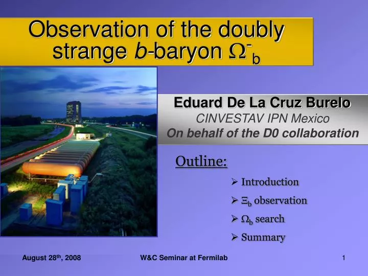
Observation of the doubly strange b- baryon - b. Eduard De La Cruz Burelo CINVESTAV IPN Mexico On behalf of the D0 collaboration. Outline: Introduction b observation b search Summary. August 28 th , 2008. W&C Seminar at Fermilab. 1. The - (sss) discovery (1964).

E N D
Observation of the doubly strangeb-baryon-b Eduard De La Cruz Burelo CINVESTAV IPN Mexico On behalf of the D0 collaboration Outline: • Introduction • b observation • b search • Summary August 28th, 2008 W&C Seminar at Fermilab 1 W&C Seminar
The -(sss) discovery (1964) The Eightfold way SU3 W&C Seminar
What energies we will looking at? Do we miss something here? Z, W, top, Higgs? Z’,W’,KK modes, etc. TeV few GeV GeV MeV W&C Seminar
What energies we will look at? B Physics Bs Mixing, CKM, lifetimes, etc. TeV few GeV GeV MeV W&C Seminar
B baryons at the Tevatron J=1/2, 1 b • Unique to Tevatron (not produced in B factories) • B baryons expected to be produced copiously at the Tevatron • Only b was considered as observed back in 2001 ~20 events. • Interesting mass predictions using different models. • However, very challenging. b(bud) b0(bud) b+(buu) b-(bdd) b0(bus) b-(bds) b-(bss) Not yet observed W&C Seminar
When Tevatron Run II begun: from hep-ph/9406359 W&C Seminar
(*)-b in October 2006 CDF announced the observation of the b’s with 1.1 fb-1 PRL 99, 202001 (2007) W&C Seminar
Last year:-b observation Number of events: 15.2 ± 4.4 Mass: 5.774 ± 0.011(stat) GeV Width: 0.037 ± 0.008 GeV We also measured: Signal Significance: PRL 99, 052001 (2007) W&C Seminar
Last year:-b observation Also searched for in b-c0- M(b-) = 5792.9 2.5 (stat) 1.7 (syst) MeV/c2 Signal significance = 7.8 PRL 99, 052002 (2007) W&C Seminar
During Tevatron Run II W&C Seminar
B hadron observation status • Mesons: • B+, B0, Bs, Bc+ (before Tevatron RunII) • B* (before Tevatron RunII) • Bd**(Tevatron RunII) • Bs** (Tevatron RunII) • Baryons: • b (before Tevatron RunII) • b+, and b*+(Tevatron RunII) • -b (Tevatron RunII) W&C Seminar
Data In this analysis we use 1.3 fb-1 of data collected by DØ detector (RunIIa data). Thanks to the Fermilab Accelerator division for doing wonderful work. Muon and central tracker subdetectors are particularly important in this analysis W&C Seminar
How did we look for the -b? -b→J/+- + - p -b - ~5 cm ~5 cm ~0.7 mm - - W&C Seminar
Data reprocessing When tracks are reconstructed, a maximum impact parameter is required to increase the reconstruction speed and lower the rate of fake tracks. p But for particles like the b-, this requirement could result in missing the and proton tracks from the and - decays W&C Seminar
Increase of reconstruction efficiency D0 D0 D0 GeV GeV GeV Opening up the IP cut: (Before) ( After ) W&C Seminar
b Reconstruction procedure • Reconstruction procedure: • Reconstruct J/→+- • Reconstruct →p • Reconstruct → + • Combine J/+ • Improve mass resolution by using an event-by-event mass difference correction • The optimization: • b→J/ decays in data • J/ + (fake from (p-)+ ) • Monte Carlo simulation of b-→J/+- Final b selection cuts: • →p decays: • pT(p)>0.7 GeV • pT()>0.3 GeV • - → decays: • pT()>0.2 GeV • Transverse decay length>0.5 cm • Collinearity>0.99 • -bparticle: • Lifetime significance>2. (Lifetime divided by its error) W&C Seminar
bss quarks combination Mass is predicted to be 5.94 - 6.12 GeV M(-b) > M(b) Lifetime is predicted to be 0.83<(-b)<1.67 ps Search for the -b(bss) W&C Seminar
How do we look for it? + - p -b - ~5 cm ~? ~3 cm - Similar K- W&C Seminar
-b vs -b: differences [1] Phys. Rev. D 77, 014031 (2008); arXiv:0708.4027 [hep-ph] (2007). [2] arXiv:hep-ph/9705402 W&C Seminar
reconstruction a challenge • →p decays: • pT(p)>0.7 GeV • pT()>0.3 GeV • - → decays: • pT()>0.2 GeV • Transverse decay length>0.5 cm • Collinearity>0.99 In this analysis for the reconstruction: D0 D0 W&C Seminar
Analysis strategy • Events are reprocessed to increase reconstruction efficiency of long-lived particles. • Select J/ candidates • Yield is optimized by using proper decay length significance cuts. • Select p • Optimize yield by using multivariate techniques • Reconstruction of → + K • Combine J/ + (K+) • Keep blinded J/ + combinations and optimize on J/ + (K+) • Improve mass resolution from 80 MeV to 34 MeV • Event per event mass correction • Perform as many test as possible in different background samples • Fix selection criteria and then apply them to J/ + W&C Seminar
optimization First we select a proper decay length significance cut to clean signal ( decay length significance > 10) D0 +K will have huge combinatory background W&C Seminar
Minimum selection cuts: +K vertex reconstructed Transverse decay length significance>4 Proper decay length uncertainty<0.5 cm reconstruction D0 PDG mass value Wrong-sign events +K+ Right-sign events (+K-) W&C Seminar
All variables are related to - or its decay products. We use a total of 20 variables. For training we use MC signal and background from wrong-sign events (J/(K+)). Most important variables: pT(K) pT(p) pT() - transverse decay length Boosted Decision Trees (BDT) W&C Seminar
- after BDT selection D0 Clean - signal W&C Seminar
This is a reflection contamination due to mistaken a pion as a kaon. It is easy to eliminate by requiring M()>1.34. -- contamination D0 D0 W&C Seminar
- after BDT selection decays removed D0 Wrong-sign combination events W&C Seminar
Final optimization • We want to further reduce background (based on level we observe in the wrong-sign combinations.) • We use - yield in MC signal verify that we maintain the highest possible signal efficiency. W&C Seminar
We compare MC signal vs wrong-sign background events pT distribution. Final optimization: pT(B)>6 GeV W&C Seminar
Similarly, MC signal is compare with uncertainty from wrong-sign events. Lxy B decay Vertex Primary vertex Final optimization: ()<0.03 cm Uncertainty on W&C Seminar
Wrong-sign combinations • After optimization: • <0.03 cm • J/ and in the same hemisphere • pT(J/+)>6 GeV • We define mass as: • Mass window for the search: 5.6 - 7 GeV After optimization, we look at wrong-sign combination first W&C Seminar
Other control sample We analyze candidates in the sidebands of - signal D0 W&C Seminar
Other control sample We analyze candidates in the sidebands of signal D0 W&C Seminar
Nothing where nothing should be We check also high statistics MC samples No excess is observed in any control samples after selection criteria is applied to them. W&C Seminar
Looking at right-sign combinations Clear excess of events near 6.2 GeV W&C Seminar
Mass measurement • Fit: • Unbinned extended log-likelihood fit • Gaussian signal, flat background • Number of background/signal events are floating parameters Number of signal events: 17.8 ± 4.9 Mean of the Gaussian: 6.165 ± 0.010(stat) GeV Width of the Gaussian fixed (MC): 0.034 GeV W&C Seminar
Significance of the peak • Two likelihood fits are performed: • Signal + background hypothesis (LS+B) • Only background hypothesis (LB) • We evaluate the significance: • Significance of the observed signal: 5.4 W&C Seminar
Consistency check: Increase pT(B) Significance >6 W&C Seminar
Consistency check: Look back plots D0 D0 W&C Seminar
Consistency check: lifetime We compare to a MC sample with a lifetime of 1.54 ps (~460 microns). W&C Seminar
Alternative Cuts Based Analysis (CBA) Variables selected based on relative importance in BDT performance W&C Seminar
Cut Based Analysis fit • Fit: • Unbinned extended log-likelihood fit • Gaussian signal, flat background • Number of background/signal events are floating parameters Number of signal events: 15.7 ± 5.3 Mean of the Gaussian: 6.177 ± 0.015(stat) GeV Width of the Gaussian fixed (MC): 0.034 GeV Signal significance: 3.9 W&C Seminar
BDT or Cut Base Analysis • After we remove duplicate events, we observe 25.5 ± 6.5 events. • Significance: 5.4 W&C Seminar
Signal confirmed without BDT • BDT vs CBA • Consistent number of observed signal candidates • Consistent mass • Consistent reconstruction efficiencies • BDT has better background rejection power. W&C Seminar
One example: Event display W&C Seminar
One example: Event display W&C Seminar
Systematic uncertainties on the mass • Fitting models • Linear background instead of flat. Negligible. • Varying Gaussian width between 28 – 40 MeV, 3 MeV • Momentum scale correction: • Fit to the b mass peak in data, 4 MeV. • Event selection: • Varying selection criteria and from the mass shift observed between the cut-based and BDT analysis, a 12 MeV variation is estimated . W&C Seminar
Production rate The systematic uncertainty includes contributions from the signal yields as well as selection efficiencies W&C Seminar
Production rate W&C Seminar
Summary Number of signal events: 17.8 ± 4.9 (stat) ± 0.8(syst) Mass: 6.165 ± 0.010(stat) ± 0.013(syst)GeV Significance= 5.4 W&C Seminar