Download
1 / 44
450 likes | 476 Views
Learn about boosting algorithms in ensemble learning, including Bagging and Boosting methods, with a focus on ADABoost. Explore weight updating, Adaboost comparison results, and practical applications in insect recognition.

E N D
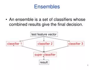
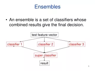
Ensembles • An ensemble is a set of classifiers whose combined results give the final decision. test feature vector classifier 1 classifier 2 classifier 3 super classifier result
MODEL* ENSEMBLES • Basic Idea • Instead of learning one model • Learn several and combine them • Often this improves accuracy by a lot • Many Methods • Bagging • Boosting • Stacking *A model is the learned decision rule. It can be as simple as a hyperplane in n-space (ie. a line in 2D or plane in 3D) or in the form of a decision tree or other modern classifier.
Bagging • Generate bootstrap replicates of the training set by sampling with replacement • Learn one model on each replicate • Combine by uniform voting
Boosting • Maintain a vector of weights for samples • Initialize with uniform weights • Loop • Apply learner to weighted samples • Increase weights of misclassified ones • Combine models by weighted voting
Boosting In More Detail(Pedro Domingos’ Algorithm) • Set all E weights to 1, and learn H1. • Repeat m times: increase the weights of misclassified Es, and learn H2,…Hm. • H1..Hm have “weighted majority” vote when classifying each test Weight(H)=accuracy of H on the training data
ADABoost • ADABoost booststhe accuracy of the original learning algorithm. • If the original learning algorithm does slightly better than 50% accuracy, ADABoost with a large enough number of classifiers is guaranteed to classify the training data perfectly.
ADABoost Weight Updating(from Fig 18.34 text) /* First find the sum of the weights of the misclassified samples */ for j = 1 to N do /* go through training samples */ if h[m](xj) <> yj then error <- error + wj /* Now use the ratio of error to 1-error to change the weights of the correctly classified samples */ for j = 1 to N do if h[m](xj) = yj then w[j] <- w[j] * error/(1-error)
Example • Start with 4 samples of equal weight .25. • Suppose 1 is misclassified. So error = .25. • The ratio comes out .25/.75 = .33 • The correctly classified samples get weight of .25*.33 = .0825 .2500 .0825 .0825 .0825 What’s wrong? What should we do? We want them to add up to 1, not .4975. Answer: To normalize, divide each one by their sum (.4975).
Sample Application: Insect Recognition Doroneuria (Dor) Using circular regions of interest selected by an interest operator, train a classifier to recognize the different classes of insects.
Boosting Comparison • ADTree classifier only(alternating decision tree) • Correctly Classified Instances 268 70.1571 % • Incorrectly Classified Instances 114 29.8429 % • Mean absolute error 0.3855 • Relative absolute error 77.2229 %
Boosting Comparison AdaboostM1 with ADTree classifier • Correctly Classified Instances 303 79.3194 % • Incorrectly Classified Instances 79 20.6806 % • Mean absolute error 0.2277 • Relative absolute error 45.6144 %
Boosting Comparison • RepTree classifier only(reduced error pruning) • Correctly Classified Instances 294 75.3846 % • Incorrectly Classified Instances 96 24.6154 % • Mean absolute error 0.3012 • Relative absolute error 60.606 %
Boosting Comparison AdaboostM1 with RepTree classifier • Correctly Classified Instances 324 83.0769 % • Incorrectly Classified Instances 66 16.9231 % • Mean absolute error 0.1978 • Relative absolute error 39.7848 %
References • AdaboostM1: Yoav Freund and Robert E. Schapire (1996). "Experiments with a new boosting algorithm". Proc International Conference on Machine Learning, pages 148-156, Morgan Kaufmann, San Francisco. • ADTree: Freund, Y., Mason, L.: "The alternating decision tree learning algorithm". Proceeding of the Sixteenth International Conference on Machine Learning, Bled, Slovenia, (1999) 124-133.
Random Forests • Tree bagging creates decision trees using the bagging technique. The whole set of such trees (each trained on a random sample) is called a decision forest. The final prediction takes the average (or majority vote). • Random forests differ in that they use a modified tree learning algorithm that selects, at each candidate split, a random subset of the features.
Back to Stone Flies Random forest of 10 trees, each constructed while considering 7 random features. Out of bag error: 0.2487. Time taken to build model: 0.14 seconds Correctly Classified Instances 292 76.4398 % (81.4 with AdaBoost) Incorrectly Classified Instances 90 23.5602 % Kappa statistic 0.5272 Mean absolute error 0.344 Root mean squared error 0.4069 Relative absolute error 68.9062 % Root relative squared error 81.2679 % Total Number of Instances 382 TP Rate FP Rate Precision Recall F-Measure ROC Area Class 0.69 0.164 0.801 0.69 0.741 0.848 cal 0.836 0.31 0.738 0.836 0.784 0.848 dor WAvg. 0.764 0.239 0.769 0.764 0.763 0.848 a b <-- classified as 129 58 | a = cal 32 163 | b = dor
More on Learning • Neural Nets • Support Vectors Machines • Unsupervised Learning (Clustering) • K-Means • Expectation-Maximization
Neural Net Learning • Motivated by studies of the brain. • A network of “artificial neurons” that learns a function. • Doesn’t have clear decision rules like decision trees, but highly successful in many different applications. (e.g. face detection) • We use them frequently in our research. • I’ll be using algorithms from http://www.cs.mtu.edu/~nilufer/classes/cs4811/2016-spring/lecture-slides/cs4811-neural-net-algorithms.pdf
Simple Feed-Forward Perceptrons in = (∑ Wj xj) + out = g[in] x1 W1 out g is the activation function It can be a step function: g(x) = 1 if x >=0 and 0 (or -1) else. It can be a sigmoid function: g(x) = 1/(1+exp(-x)). g(in) x2 W2 The sigmoid function is differentiable and can be used in a gradient descent algorithm to update the weights.
Gradient Descenttakes steps proportional to the negative of the gradient of a function to find its local minimum • Let X be the inputs, y the class, W the weights • in = ∑ Wjxj • Err = y – g(in) • E = ½ Err2 is the squared error to minimize • E/Wj = Err * Err/Wj= Err * /Wj(g(in))(-1) • = -Err * g’(in) * xj • The update is Wj <- Wj + α * Err * g’(in) * xj • α is called the learning rate.
Simple Feed-Forward Perceptrons repeat for each e in examples do in = (∑ Wj xj) + Err = y[e] – g[in] Wj = Wj + α Err g’(in) xj[e] until done x1 W1 out g(in) x2 W2 Examples: A=[(.5,1.5),+1], B=[(-.5,.5),-1], C=[(.5,.5),+1] Initialization: W1 = 1, W2 = 2, = -2 Note1: when g is a step function, the g’(in) is removed. Note2: later in back propagation, Err * g’(in) will be called Note3:We’ll let g(x) = 1 if x >=0 else -1
Graphically Examples: A=[(.5,1.5),+1], B=[(-.5,.5),-1], C=[(.5,.5),+1] Initialization: W1 = 1, W2 = 2, = -2 W2 Boundary is W1x1 + W2x2 + = 0 wrong boundary A C B W1
Examples: A=[(.5,1.5),+1], B=[(-.5,.5),-1], C=[(.5,.5),+1] Initialization: W1 = 1, W2 = 2, = -2 repeat for each e in examples do in = (∑ Wjxj) + Err = y[e] – g[in] Wj = Wj + α Err g’(in) xj[e] until done Learning A=[(.5,1.5),+1] in = .5(1) + (1.5)(2) -2 = 1.5 g(in) = 1; Err = 0; NO CHANGE B=[(-.5,.5),-1] In = (-.5)(1) + (.5)(2) -2 = -1.5 g(in) = -1; Err = 0; NO CHANGE • Let α=.5 • W1 <- W1 + .5(2) (.5) leaving out g’ • <- 1 + 1(.5) = 1.5 • W2 <- W2 + .5(2) (.5) • <- 2 + 1(.5) = 2.5 • <- + .5(+1 – (-1)) • <- -2 + .5(2) = -1 C=[(.5,.5),+1] in = (.5)(1) + (.5)(2) – 2 = -.5 g(in) = -1; Err = 1-(-1)=2
Graphically Examples: A=[(.5,1.5),+1], B=[(-.5,.5),-1], C=[(.5,.5),+1] Initialization: W1 = 1, W2 = 2, = -2 W2 a Boundary is W1x1 + W2x2 + = 0 wrong boundary A C B W1 approximately correct boundary
p1 vector W b error new W
Back Propagation • Simple single layer networks with feed forward learning were not powerful enough. • Could only produce simple linear classifiers. • More powerful networks have multiple hidden layers. • The learning algorithm is called back propagation, because it computes the error at the end and propagates it back through the weights of the network to the beginning.
(slightly different from text) Let’s break it into steps.
Let’s dissect it. layer 1 2 3=L w11 x1 w1f n1 w21 nf x2 w31 w2f n2 x3
Forward Computation layer 1 2 3=L w11 x1 n1 w1f w21 nf x2 w31 w2f n2 x3
Backward Propagation 1 • Node nf is the only node in our output layer. • Compute the error at that node and multiply by the • derivative of the weighted input sum to get the • change delta. layer 1 2 3=L w11 x1 n1 w1f w21 nf x2 w31 w2f n2 x3
Backward Propagation 2 • At each of the other layers, the deltas use • the derivative of its input sum • the sum of its output weights • the delta computed for the output error layer 1 2 3=L w11 x1 n1 w1f w21 nf x2 w31 w2f n2 x3
Backward Propagation 3 Now that all the deltas are defined, the weight updates just use them. layer 1 2 3=L w11 x1 n1 w1f w21 nf x2 w31 w2f n2 x3
Back Propagation Summary • Compute delta values for the output units using observed errors. • Starting at the output-1 layer • repeat • propagate delta values back to previous layer • update weights between the two layers • till done with all layers • This is done for all examples and multiple epochs, till convergence or enough iterations.
Time taken to build model: 16.2 seconds Correctly Classified Instances 307 80.3665 % (did not boost) Incorrectly Classified Instances 75 19.6335 % Kappa statistic 0.6056 Mean absolute error 0.1982 Root mean squared error 0.41 Relative absolute error 39.7113 % Root relative squared error 81.9006 % Total Number of Instances 382 TP Rate FP Rate Precision Recall F-Measure ROC Area Class 0.706 0.103 0.868 0.706 0.779 0.872 cal 0.897 0.294 0.761 0.897 0.824 0.872 dor W Avg. 0.804 0.2 0.814 0.804 0.802 0.872 === Confusion Matrix === a b <-- classified as 132 55 | a = cal 20 175 | b = dor