Download
1 / 66
660 likes | 666 Views
3 Causal Models Part III: DAGs and new approaches to bias. Matthew Fox Advanced Epidemiology. Discussion: How do we decide what are potential candidates for an adjusted model?. Multivariate modeling example.

E N D
3 Causal Models Part III:DAGs and new approaches to bias Matthew Fox Advanced Epidemiology
Discussion: How do we decide what are potential candidates for an adjusted model?
Discussion: If a variable is not a confounder is it reasonable to include it in a model to see its effect on the outcome as well?
This Morning • Counterfactual model • 4 types: doomed, causal, preventive, immune • Emphasize role of reference group • No confounding as partial exchangeability • Separate from confounders • p1 + p3 = q1 + q3 • Non-identifiably leads to collapsibility • If crude = adjusted, collapse • Mantel-Haenszel if no interaction, SMR if yes • Odds ratio is not strictly collapsible • Statistical criteria can fail
Approaches to Confounding • Multivariable analysis • Limits of statistical criteria • Which variables are candidates for a model? • Directed acyclic graphs • Visual approaches to detecting and adjusting for confounding • Direct and Indirect effects • The structural nature of bias
Multivariate modeling – Conventional Epi Approach • To identify set of variables to include: • Add largest confounder influence > criterion (10%) • RRc <0.9 or >1.1 • Stepwise, but based on change in estimate • Add next largest, if ∆ still > 10%, add next largest • Stop when the change is below 10% • Political variables? • Never a question of statistical significance • We are interested in the effect of an exposure • A variable may predict outcome, but not confound • In this case we typically just lose power
Problems with statistical approach • Ignores everything we know about the relationship between variables in the model • Removes control and thought • Can go wrong when causal structure is complicated • And it often is complicated • What is a better approach for identifying an appropriate set of confounders? • Causal diagrams
Common Causes E C D What is it? If no effect of E on D, will E and D be associated if we do nothing? Does E cause D?
Indirect Effect C E D If we do nothing, will E and D be associated? Does E cause D?
Common effects E C D If E doesn’t cause D, if we do nothing, will E and D be associated? Will E and D be associated with C? Would stepwise procedures include it?
Terminology - DAGs • Arc or Edge • Line connecting two variables • Arrows encode causal relations • No arrow = independence • Arrows indicate the flow of information • Parent-Child • Arrow from one node to another • Ancestor E C D B
Terminology - DAGs • Directed: • All parent to child • Acyclic: • No directed path forms a loop • Future cannot predict the past • Causal: • All arrows represent effects E C D B
Adopt convention time flows from left to right. Heads of arrows should always be to right of tails
Terminology - DAGs • A path • Unbroken route • Directed path • Always leaving tail, entering a head • Backdoor path • A non-causal path from E to D that does not contain any variable affected by E • Collider • Can’t go in 1 arrow head & out 2nd head • Specific to a path • Blocked path • A path is blocked if there is a collider • Or we control for a variable on the path
Causal DAGs • An arrow implies an effect • A→Y means Pr[Ya=1=1]≠ Pr[Ya=0=1] • A DAG is causal if the common causes of any two variables are shown in the graph • In other words, does not need to include every variable • Start with E and D and look for all common causes • Then add common causes of those variables • Common causes imply association not causation
We use DAGs to see if two variables are d-separated • D = “directional” • D-separation means we can determine causality • If our DAG is “faithful” • A and B will be d-separated if there is no unblocked backdoor path from A to B • Unconditional independence • Two variables will also be d-separated if all paths are blocked through control • Conditional independence
DAGs show association and causation • The DAG, if causal, says: • Pr[Ya=1=1] = Pr[Ya=0=1] and • Pr[Y=1|A=1] ≠ Pr[Y=1|A=0] • In other words: • A does not cause Y, so the true effect of A on Y is null • In our crude data, A will be associated with Y No Causation Association C Y A
DAGs show association and causation • The DAG, if causal, says: • Pr[Yc=1=1] ≠ Pr[Yc=0=1] and • Pr[Y=1|C=1] ≠ Pr[Y=1|C=0] • In other words: • C does cause Y, so the true effect of C on Y is not null • In our crude data, the association between C and Y will be the causal effect Causation Association C Y A
DAGs show association and causation • The DAG, if causal, says: • Pr[Ac=1=1] ≠ Pr[Ac=0=1] and • Pr[A=1|C=1] ≠ Pr[A=1|C=0] • In other words: • C does cause A, so the true effect of C on A is not null • In our crude data, the association between C and A will be the causal effect Causation Association C Y A
General Rule of DAGs:We can trace a backdoor path from E to D going in any direction we like, except we can’t go in the head of one arrow and out the head of another or through a variable we control for statistically.
Rules of DAGs • A path is blocked if: • It contains a non-collider that’s been conditioned on • OR: It contains a collider not conditioned on and no child of that collider has been conditioned on • Conditioning on a child partly conditions on the parent • Two variables are d-separated if all backdoor paths between them are blocked • No confounding
To diagnose confounding, firstremove all arrows emanating from E
Estimates of the effect of E on Dwill be confounded if there is an unblocked backdoor path from E to D
Note that each path we can trace really shows common causes – look again. Confounding IS common causes.
Conditioning on a collider • Conditioning on a collider opens the flow of information • Only two reasons the ground can be wet • It can rain • Sprinkler is on 1 week schedule • Unrelated to weather • The two are completely unrelated Sprinkler Rain Ground is wet
Conditioning on a collider • We notice the ground is wet • This is equivalent to only looking in the strata wet = 1 • If we know it rained, is it more or less likely that the sprinkler was on? • If we know the sprinkler was on, is it more or less likely that it rained? Sprinkler Age Rain Ground is wet
As an example • If 50% chance of rain and 50% chance of sprinkler on, and both are independent: • If rain, chance of sprinkler is 50% • If no rain, chance of sprinkler is 50%, RR = 1 • If I wake up and the ground is dry: • Perfect correlation (both did not occur) • If I wake up and ground is wet then: • If rain, chance of sprinkler on is 50% • If no rain, chance of sprinkler on is 100%, RR = 2 • If sprinkler was on, chance of rain is 50% • If sprinkler was off, chance of rain is 100%, RR = 2
Put another way • If we had two independent variables that perfectly predicted a third • A and B are independent binary variables and • C = A + B • Then • If we look among C = 2, A and B must be 1 • If we look among C = 0, A and B must be 0 • If we look among C = 1, if A = 1 then B = 0 and if A = 0, C = 1 • So within C, A & B are perfectly correlated
Ways two variables can be associated • Causation • Direct, indirect and reverse • Common causes • Conditioning on a common effect • Random variation • Not a part of DAGs which represent structural relations
Circumcision and HIV DAG Age Religion # sexual partners Circumcision HIV
Circumcision and HIV DAG:Remove arrows from exposure Age Religion # sexual partners Circumcision HIV
Circumcision and HIV DAG: Any unblocked backdoor paths? Age Religion # sexual partners Circumcision HIV
Circumcision and HIV DAGNew paths? Age Religion # sexual partners Circumcision HIV
Circumcision and HIV DAGNew paths Age Religion # sexual partners Circumcision HIV
Circumcision and HIV DAGIdentify {S} (sufficient set?) Age Religion # sexual partners Circumcision HIV
Circumcision and HIV DAGNew paths? Age Religion # sexual partners Circumcision HIV
Circumcision and HIV DAGAll unblocked paths pass {S}? Age Religion # sexual partners Circumcision HIV
Which is the confounder, age or sexual partners? Age Religion # sexual partners Circumcision HIV
Could also have just chosen religion Age Religion # sexual partners Circumcision HIV