Download
1 / 72
720 likes | 831 Views
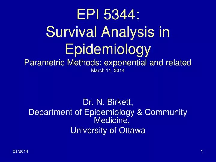
EPI 5344: Survival Analysis in Epidemiology Parametric Methods: exponential and related March 11, 2014. Dr. N. Birkett, Department of Epidemiology & Community Medicine, University of Ottawa. Objectives. Introduce the Accelerated Failure Time model The simple exponential model and MLE

E N D
EPI 5344:Survival Analysis in EpidemiologyParametric Methods: exponential and relatedMarch 11, 2014 Dr. N. Birkett, Department of Epidemiology & Community Medicine, University of Ottawa
Objectives • Introduce the Accelerated Failure Time model • The simple exponential model and MLE • Iterative methods to estimate MLEs • The piece-wise exponential model. • Using likelihood ratio methods to compare models
Intro (1) • Parametric methods are not commonly used in epidemiology • Exponential and piece-wise exponential are exceptions. • Based on an Accelerated Failure Time (AFT) model • Like saying that one year of a dog’s life counts as 7 human years.
Intro (1a) • The time at which survival in my study group is the same as survival in the reference group at time ‘t0’ is: • Survival in my study group at time ‘t’ is the same as survival in the reference group at time ‘R*t’:
TR = 2.0 Curve 1 has longer survival Curve 2 Curve 1
Intro (2) • We model the ‘event time’ directly:
Intro (3) • Similar to linear regression (show on board) • εi is a random variable • assumed constant mean and variance over all subjects • can assume any of a range of distributions • Normal Dist’n ‘T’ follows log-normal dist’n • σ is scale parameter • Can be used to test assumptions about shape of εi • ‘Scales’ random error distribution
Intro (4) • AFT and PH assumptions are separate • Some models have both properties but most don’t • exponential and Weibull are both AFT and PH • Time Ratio (TR) and Hazard Ratio (HR) • TR gives the increase in survival time for exposures • HR gives the increase in hazard (risk) • If TR is >1.0, HR will be <1.0 • Can convert between them if we know the math • SAS use Proc Lifereg to fit parametric models
Exponential Model (1) • Hazard is constant:
Exponential Model (2) • Consider two groups with exponential survival: • How does the survival of group 1 relate to group 0? Accelerated Failure Time Model
Exponential Model (4) • The AFT models and PH model with constant hazard are equivalent • Beta from one model is negative of beta from other model • Doesn’t matter if we use hazard or AFT approach • I will stick with hazards • For constant hazard model, εi is the ‘Extreme value’ distribution
Exponential Model (5) • If HR >1, then study group has events which happen earlier in time • Same effect as TR<1 • Since hazard is constant, then we have:
Exponential Model (6) • How do we estimate λ? • Use MLE • Means that we need a likelihood function • Slightly different from previous session since we have continuous distributions • Prob(event time=any ‘t’) = 0 • Instead, use the probability density function • f(t)
Exponential Model (7) • Two types of events (ends) can happen: • Death • Censored • Each contribute to the likelihood function but in different ways
Exponential Model (8) • Likelihood contribution of a death at time ti: • Likelihood contribution if censored at time : • Actual time of ‘failure’ is unknown. • Must survive until at least time • Multiply these across all deaths and all censored events to get full likelihood
Exponential Model (10) • How do we find the MLE for λ?
Exponential Model (11) • How can we check if the data follows the exponential model? • This gives a straight-line y=a+bx. Where:
Exponential Model (12) • Complementary log-log plot • Plot ‘log(-log(S(t))’ vs. ‘log(t)’ • Look for a straight line. • Later on, this plot will prove very useful for testing proportional hazard assumption.
Exponential Model (13) • What if we want to examine predictors of the outcome? • λ is allowed to vary by sex, age, cholesterol, etc. • Use the same approach but now, instead of a fixed ‘λ’, we use the following in the likelihood function:
Exponential Model (14) • We need to find an MLE for each of the Betas. • There is NO closed form formula to solve this case! • Must use iterative methods to estimate each of the Betas. • Approach used in ALL real MLE-based analyses • Computers are very good at doing this.
Guess #3 Guess #1 Guess #2
Exponential Model (15) • Real algorithm is more sophisticated. • Usually converges in 4-5 steps. • HOWEVER, it: • May take longer or • May never converge
Uses recidivism data set libname allison 'C:/allison_2010/data_sets'; ODS GRAPHICS ON; ods rtf; PROC LIFEREG DATA=allison.recid; MODEL week*arrest(0)=fin age race wexp mar paro prio / DISTRIBUTION=exponential; RUN; ODS rtf close; ODS GRAPHICS OFF;
Financial aid effect • Seems to imply financial aid makes things worse! • But, last week we found that financial aid reduced the rate of recidivism. • This is NOT the hazard ratio. • LIFEREG gives the Time Ratio.
Lagrange Multiplier section • Formally, tests if the ‘scale’ parameter (σ) is ‘1’ • ‘σ’ relates to Weibull distribution • If ‘σ’=1, Weibull becomes the exponential. • If ‘σ’≠1, then hazard is not constant over time. • Informally, use this as a test that the hazard is constant.
‘CLASS’ statement in SAS (1) • Education measures highest grade completed. • Grouped into five levels: • 6th grade or lower • 7th to 9th grade • 10th to 11th grade • 12th grade • some college • Coded as 2/3/4/5/6
‘CLASS’ statement in SAS (2) • How to model? • Include in ‘model’ statement • treated as continuous • same change in risk from level 2 to 3 as from 5 to 6, etc. • not a good approach. • ordinal variable • include as dummy variables • Could code yourself in a Data step • Better: use the ‘class’ statement in SAS
libname allison 'C:/allison_2010/data_sets'; ODS GRAPHICS ON; ods rtf; PROC LIFEREG DATA=allison.recid; CLASS educ; MODEL week*arrest(0)=fin educ / DISTRIBUTION=exponential; RUN; ODS rtf close; ODS GRAPHICS OFF;
Exponential Model (16) • Exponential is only one model • Could also use: • Weibull • log-normal • log-logistic • Gamma • etc.
Piecewise Exponential Model (1) • Hazard is rarely constant over follow-up time • A better approximation can be found using piecewise exponential models • Divide follow-up time into intervals • The hazard is assumed constant within interval • Can vary between intervals. • Useful in the ‘real world’ where event times are often not very precisely known
Piecewise Exponential Model (2) • Lifereg allows you to test hypotheses about the hazard directly. • Start by dividing follow-up time into a set of ‘J’ intervals (they need not be the same size) • Cut-points:
a2 a3 a4 a0 a1
Piecewise Exponential Model (3) • The hazard for individual ‘i’ is of the form: • Or, we could write: • Where: • This is the same as the exponential model except that the hazard is allowed to vary during follow-up time • If we include some predictors, model becomes:
Piecewise Exponential Model (4) • The hazard for individual ‘i’ is of the form: • Or, we could write: • Where: • Easy to estimate these models with SAS. • Need data in the ‘right’ format
Piecewise Exponential Model (5) • To-date, data has one record per subject. • Each record contains • Time of event • Type of event • Covariates • For piece-wise model, each subject needs one record for each interval. • Time spent interval • Type of event in this interval • Covariates
Recidivism data (first 9cases) Obs week arrest fin age race wex mar paro prio 1 20 1 0 27 1 0 0 1 3 2 17 1 0 18 1 0 0 1 8 3 25 1 0 19 0 1 0 1 13 4 52 0 1 23 1 1 1 1 1 5 52 0 0 19 0 1 0 1 3 6 52 0 0 24 1 1 0 0 2 7 23 1 0 25 1 1 1 1 0 8 52 0 1 21 1 1 0 1 4 52 0 0 22 1 0 0 0 6 • Allow hazard to vary in each quarter of the year: • 0-12+ • 13-25+ • 26-38+ • 39-51+ • Need to re-structure table to give one record per subject per quarter. • Ignore covariates for now • Consider subject #1
Piece-wise Exponential Model (6) • Subject was re-arrested in week 20 • Quarter #2. • What will the new data look like? • One record for quarters 1 & 2. • No record for quarters 3 & 4
Recidivism data (first 9cases) Obs week arrest fin age race wex mar paro prio 1 20 1 0 27 1 0 0 1 3 2 17 1 0 18 1 0 0 1 8 3 25 1 0 19 0 1 0 1 13 4 52 0 1 23 1 1 1 1 1 5 52 0 0 19 0 1 0 1 3 6 52 0 0 24 1 1 0 0 2 7 23 1 0 25 1 1 1 1 0 8 52 0 1 21 1 1 0 1 4 52 0 0 22 1 0 0 0 6
Piece-wise Exponential Model (7) • Subject was never re-arrested. • What will the new data look like? • One record for each quarter
Piece-wise Exponential Model (8) • Main challenge is technical • How to re-structure the SAS data set? • How to describe new data layout to SAS?
Piece-wise Exponential Model (9) DATA quarter; SET allison.recid; quarter=CEIL(week/13); DO j=1 TO quarter; time=13; event=0; IF (j=quarter AND arrest=1) THEN DO; event=1; time=week-13*(quarter-1); END; OUTPUT; END; RUN;