Download
1 / 59
610 likes | 898 Views
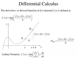
DIFFERENTIAL CALCULUS. Outcomes for this session. By the end of this session, you should be able to: Develop an intuitive understanding of the limit concept, in the context of approximating the rate of change or gradient of a function at a point.

E N D
Outcomes for this session • By the end of this session, you should be able to: • Develop an intuitive understanding of the limit concept, in the context of approximating the rate of change or gradient of a function at a point. • Determine the average gradient of a curve between two points, i.e.: m = • Determine the gradient of a tangent to a graph, which is also the gradient of the graph at that point. Introduce the limit principle by shifting the secant until it becomes a tangent. • Use first principles for (x) = for f(x) = k ; f(x) = ax and • f(x) = ax2+ b. • Use the rule for n • Find equations of tangents to graphs of functions. • Sketch graphs of cubic polynomial functions using differentiation to determine the co-ordinate of stationary points. Also, determine the x-intercepts of the graph using the factor theorem and other techniques. • Solve practical problems concerning optimization and rates of change, including calculus of motion.
Introduction • Calculus is a branch of mathematics involving or leading to calculations dealing with continuously varying functions. • To a Roman in the days of the empire a “calculus” was a pebble used in counting and gambling. • Centuries later “calculare” came to mean “to compute”, “to reckon”, “to figure out”. To the mathematician, physical scientist, and social scientist of today, calculus is elementary mathematics (algebra, geometry, trigonometry) enhanced by the limit process. • Calculus takes ideas from elementary mathematics and extends them to a more general situation. • The table below contains some examples. On the left-hand side, you will find an idea from elementary mathematics; on the right, this same idea as extended by calculus
Gradient of a curve Notice that at point A the gradient is positive and at point B the gradient is negative. In general terms, we define the gradient of a curve at a given point, say P(x ; y), to be the gradient of the tangent line to the curve at the point P.
Intuitive definition of a limit • Let f be a function which is defined for all of x “near” x = a. If, as x tends to a from both the left and from the right, f(x) tends to a number, say b, then we say that the limit of f(x), as x tends to a is b. • We write: = bORf(x)b as x a • We say nothing about f (a). Perhaps f (a) exists and perhaps it doesn’t. And if it does, perhaps = f (a) and perhaps not! • When dealing with limits we only care about where we are going, not whether we get there!
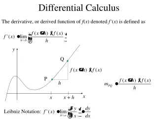
Differentiation from first principles • is the same as and is called the differential coefficient or the derivative. The process of finding the differential coefficient is called differentiation. • To summarise: The differential coefficient • = = • =
Rules of differentiation • To calculate the derivative of ,say f(x) = xgoogle, from first principles may be a daunting task to the ordinary human being. To assist in accomplishing this and other similar tasks, rules for differentiation have been developed and accepted. • Suppose that y = xn, where n is a real number Then = nxn–1
Acceptable notations • The following are the commonly used symbols depicting differentiation of a function. • Symbols instructing differentiation are : or D; • Symbols indicating differentiation to the variable x are: or Dx ; • Differentiation with respect to the variable y are indicated by: or Dy ; • Differentiation of f(x) with respect to x are indicated by: • f(x) or or Dx[f(x)] or (x) • Differentiation of y with respect to x are indicated by: • y or or Dx[y] or
Equations of tangents to graphs • The derivative also results in the gradient of a tangent to a function. For example, if we differentiate the equation of a curve, we will get the formula for the gradient of the curve at a point, and thus the gradient of a tangent to the curve at that point. • We can then proceed to calculate the equation of a tangent to the curve at that point.
Activity 7: Equation of tangent to a curve at a given point.
Activity 7: Equation of tangent to a curve at a given point.
Summary (How to find the equation of a tangent touching a curve at a point where x = k) • Determine . This gives you the gradient function. • Next calculate . This gives you the actual gradient at that point, x = k. • Find f(k), the y-coordinate of the “touching point”. • Let the equation of the tangent be y = mx +c. Substitute m (the gradient); k (the x-value) and f(k) (for the y-value) to calculate c. • Write down the equation of the tangent.
Steps to follow when sketching cubic functions : y = ax3 + bx2 + cx + d ; a 0
Worked example: Sketching of a cubic function • Sketch the graph of . Clearly indicate the intercepts with the axes as well as the turning points.
Some important terms…. It is important to understand the notation used in this section of Mathematics. To sketch a cubic function can be asked without giving the actual function. Important information regarding the function will be given which will have to be interpreted carefully before the graph can be drawn.
Activity: Sketching of cubic functions 1. Given: • Calculate the coordinates of the turning points of . • Calculate the coordinates of the x–intercepts. • Sketch the graph of , clearly indicating the intercepts with the axes and the turning points. • For which values of x will ? • Determine the equation of a tangent to the curve at the point . 2. Given: • Calculate and hence determine the x–intercepts of . • Determine the turning points of . • Sketch the graph of . Clearly show the intercepts with the axes and also the stationary points. • Write down the value of x for which .