Download
1 / 31
310 likes | 456 Views
Bias Correction of RTFDDA Surface Forecasts. Presented by: Daran Rife National Center for Atmospheric Research Research Applications Laboratory Boulder, Colorado 26 July 2006. Why implement a statistical correction?. Real world. Model representation. Imperfect

E N D
Bias Correction of RTFDDA Surface Forecasts Presented by: Daran Rife National Center for Atmospheric Research Research Applications Laboratory Boulder, Colorado 26 July 2006
Why implement a statistical correction? Real world Model representation • Imperfect • Small-scale features not resolved
Why Not Use a Traditional MOS Approach? • Traditional MOS requires: • A “frozen” weather forecast model (no upgrades). • Lengthy data archive for “training” MOS equations. • Implications: • MOS system must be completely “re-trained” whenever model is upgraded—difficult and very time consuming.
One Alternative Running-mean bias correction • Advantages: • Improve/upgrade model at any time. • Long data archive not needed. • Relatively easy to implement. • Significant increase in forecast accuracy.
Schematic of Point-wise Running-mean Bias Correction Bias correction computed as function of station location and time of day
Bias Correction Provided for: • 2 m AGL temperature • 2 m AGL dew point temperature • 2 m AGL relative humidity • 10 m AGL wind direction • 10 m AGL wind speed
Demo White Sands Missile Range
Outline • How does the gridded bias correction scheme work? • Example output from gridded bias correction system. • Timeline for implementing gridded bias correction scheme into ATEC operations.
Estimating Forecast Biases Between and Away from Obs Locations
How Does the Gridded Bias Correction Scheme Work? • STEP 1: Measure forecast bias at observation locations. • STEP 2: Calculate coefficients of regression that describe the linear relationship between the running-mean forecast variables at the obs locations, and those at every point on the grid.
How Does the Gridded Bias Correction Scheme Work? • STEP 1: Measure forecast bias at observation locations. • STEP 2: Calculate coefficients of regression that describe the linear relationship between the running-mean forecast variables at the obs locations, and those at every point on the grid. • STEP 3: Subtract bias from “raw” forecast to obtain a correction at each obs location. • STEP 4: Use regression coefficients to “map” to corrections (at obs sites) onto the full grid.
Diurnal Evolution of Forecast Bias 29 June 2005
How Well do Gridded Bias Estimates Fit the Observations? WSMR grid 3 area Regime changes
Bias Corrected Forecast Grids Uncorrected Forecast 1800 UTC 29 June 2005
Advantage of Gridded Bias Correction Scheme • Highly refined estimates of surface meteorological variables at all places on the range.
How Will ATEC Forecasters Benefit from Gridded Bias Correction Scheme? • Substantially more accurate forecasts (on average). • Use gridded BC to refine the GCAT climatographies that will be generated for each range.
Use BC with CAUTION During Regime changes! How Much Are Forecasts Improved Through Bias Correction? 2-m AGL temperature over WSMR grid 3.
Timeline for Implementing Gridded Bias Correction into ATEC Operations • FY06: Implement at ATC and DPG. • FY07: Implement at other ranges where RTFDDA running.
Display of Bias Corrected Forecasts • Web-based “Tabular Sites Data” tool • Web-based “FDDA Image Viewer”. • JViz?
Future Plans • FY07-FY08: Develop/test method to bias correct the full 3D forecast grid.
Intelligent Use of Model Output • Know the limitations of the model • General limitations of NWP models: • Does not properly treat thin cloud layers. • Cannot adequately represent shallow nocturnal boundary layers (or shallow inversions). • Solutions near grid boundaries should be used with caution. • Models under-estimates the true amount of atmospheric variability (both spatial and temporal).
Limitations of NWP Models Continued) • Does not account for shadows cast by terrain. • Very-small-scale landscape features, such as a narrow canyon outlet or mountain pass, are not represented well (or at all) by the model. • The model does not predict the production, movement, and concentration of atmospheric aerosols. Thus, it can’t predict dust storms or how plumes of airborne dust will impact the sensible weather. Same thing is true for smoke plumes from forest fires. These deficiencies lead to errors in the forecast. To the extent that these errors are systematic, the bias correction scheme can be used to remove them.
Intelligent Use of Model Output • Situations where the model output should be more closely scrutinized: • Does model snowfall/rainfall accumulation correspond well with what was observed? • Moist convection is very hard to predict. • The PBL conditions during the transition from daytime unstable to nighttime stable conditions (and the opposite transition) are very hard to predict.
GFS MOS Forecast for KELP EL, TX KELP GFS MOS GUIDANCE 7/19/2006 1200 UTC DT /JULY 19/JULY 20 /JULY 21 /JULY 22 HR 18 21 00 03 06 09 12 15 18 21 00 03 06 09 12 15 18 21 00 06 12 N/X 74 98 72 100 75 TMP 89 93 95 89 83 80 76 84 91 95 95 89 83 78 74 83 92 97 97 85 77 DPT 53 51 49 49 51 52 53 55 52 49 47 48 49 50 51 54 53 50 48 50 53 CLD BK BK BK SC SC FW FW CL FW BK SC SC SC SC SC SC SC SC SC SC SC WDR 06 12 09 12 09 06 04 09 10 11 11 14 11 09 06 10 07 09 09 09 03 WSP 09 10 07 06 08 06 04 05 08 09 10 07 07 06 05 05 09 11 12 08 08 P06 11 11 9 5 9 10 5 5 10 6 3 P12 14 12 11 11 6 Q06 0 0 0 0 0 0 0 0 0 0 0 Q12 0 0 0 0 0 T06 24/ 0 23/ 0 8/ 0 0/ 0 11/ 0 17/ 0 9/ 0 1/ 0 20/ 0 8/ 0 T12 37/ 0 8/ 0 17/ 0 9/ 1 29/ 0 CIG 8 8 8 8 8 8 8 8 8 8 8 8 8 8 8 8 8 8 8 8 8 VIS 7 7 7 7 7 7 7 7 7 7 7 7 7 7 7 7 7 7 7 7 7 OBV N N N N N N N N N N N N N N N N N N N N N
Why not use yesterday’s bias to correct today’s forecast? Example: Bias 11 June = +6 °C (too warm) Bias 12 June = -3.5 °C (too cold) Obs temp 12 June = 18 °C Fcst temp 12 June = 14.5 °C Correct the 12 June forecast using previous day’s (11 June) bias: BC=14.5 °C–6 °C= 8.5 °C Our goal was to correct the Forecast toward the Observation, but… We have made correction in the wrong direction! Time series of bias estimate
WSMR S05 for Aug 2003 How do we choose length of sampling period for computing bias correction? Main Goal: produce the most accurate result on average