Download
1 / 54
540 likes | 682 Views
Flows in Planar Graphs. Hadi Mahzarnia. Outline. Introduction Planar single commodity flow Multicommodity flows for C 1 Feasibility Algorithm DELTAFLOW Algorithm MULTIFLOW1 Multicommodity flows for C a Feasibility Algorithm MULTIFLOW2. Introduction. A Classic Problem:

E N D
Flows in Planar Graphs Hadi Mahzarnia
Outline • Introduction • Planar single commodity flow • Multicommodity flows for C1 • Feasibility • Algorithm DELTAFLOW • Algorithm MULTIFLOW1 • Multicommodity flows for Ca • Feasibility • Algorithm MULTIFLOW2
Introduction • A Classic Problem: • Finding the maximum flow of a single commodity in an arbitrary directed graph • The key theorem: • Max Flow-Min Cut theorem(Ford & Fulkerson) which holds for single commodity and two-commodity flow • There exist efficient algorithms( o(nm log n) ) for the classic problem
Our Situation(1) • More than two commodity • No true polynomial time algorithm is known on general graphs • Problem statements : • Test the feasibility of flows • Finding the flows • Can be formulated as a linear program, thus it can be solved by the simplex or other LP methods
Our Situation(2) • We concentrate on planar undirected graphs • It has been established that the Max Flow-Min Cut theorem of multicommodity type holds for the following four classes of planar undirected graphs
Class 1; C1 • All sources and sinks are located on a specified face boundary S1 t2 S2 t3 t1 S3
Class 2; C12 • All sources and sinks are located on two specified face boundaries with each source-sink pair on the same boundary t2 S1 t1 S2
Class 3; C01 • Some source-sink pairs are located on a specified face boundary, and all the other pairs share a common sink located on the boundary(their sources may be located anywhere) t3 S3 t4 S1 S4 t2 t1 S2
Class 4; Ca • All the sources can be joined with the corresponding sinks without violating planarity S2 S1 t1 t2
Definition • A (flow) network N=(G, P, c) is a triplet, where: • G = (V, E) is a finite undirected graph with vertex set V and edge set E; • P is the set of source-sink pairs(si, ti), where source si and sink ti are distinguished vertices. • c: E R+ is the capacity function • A network N is planar if G is planar, and is a K-network if it has K source-sink pairs
Each source-sink pair is given a nonnegative demand di ≥ 0 • Although G is undirected, we orient the edges so that the sign of a value of a flow function can indicate the real direction of the flow in an edge
A Three-commodity flow S1 t2 S2 t3 t1 S3
Planar single-commodity flow • The N is a 1-network in class Ca. • The algorithm starts with zero flow and pushes flow as much as possible through the upper-most path.
Theorem 11.1 : the uppermost path algorithm finds a maximum flow, whose value is equal to the minimum cut separating s and t. • Proof: by induction on the number of edges.
The algorithm merely executes the shortest path computation on the dual of G=(V, E) • Ga Obtained from G by adding an edge joining s and t of infinite capacity. • Let Ga*(V*, E*) be the dual of Ga. • Define a length function l on E* and potential function u on V* . • A maximum flow function f can simply be constraucted as follows: f(i,j) = u(j *) – u(i *)
S* S t t*
Multimodality flows for C1 • Preliminary: • We generically denote by B the boundary of the outer face of G. Also use B for the set of edges on B. • The boundary B is a cycle if G is 2-connected, but is a closed walk in general. • B may has some bridges in general. • Vertices on B are v0, v1, …, vbtaken in clockwise order. • Further we may assume without loss of generality that the given planar graph G is connected. • E(x,y) : set of edges between x and y with capacity c(x, y) and demand d(x,y) • E(x) = E(x, v-x) is called a cut • E(x) is a cutset If G – E(x) has exactly two connected components.
We shall compute c(e, e’) and d(e, e’) quickly • We can compute d(e, e’) for e fixed e and all e’ in o(k+b) time. These values can be easily updated for the new e next to the current e on B. Thus we can compute d(e, e’) in o(k+b2) time.
To compute the c(e, e’), first construct a new graph G* as follows: • Replace every edge on B by a pair of multiple edge. • Construct the dual of G. • Delete the outer vertex. • Define the length function using the capacities. • The minimum value of c(e, e’) in G is equal to the shortest path between vertices corresponding e and e’ in G*.
S1 t1
We can compute c(e, e’) in o(T(n)) time for a fixed e and in o(bT(n)) or o(Tall(n)) for all e. • Above all the feasibility can be tested in o(bT(n)) or o(Tall(n)) time.
DELTAFLOW terminates finitely if the capacities and demands are all integers. However this is not the case if they are real valued. • There are three obstructions to the correctness of polynomial boundedness of DELTAFLOW.
Obstructions … • If edge e0 is selected arbitrarily DELTAFLOW does not always terminates in polynomial time: when there exists an edge e of infinite capacity of the boundary b, DELTAFLOW possibly lets a flow go and return infinitely many times through e. • The number of source sink pairs increases and the representation of flow functions would require a greate deal of space. • The new graph G’ may be disconnected even if G is connected.
Algorithm MULTIFLOW1 • MULTIFLOW1 finds multicommodity flows in planar networks which spends O(kn+nT(n)) time and O(kn) space. • MULTIFLOW1 uses the operation of DELTAFLOW but is improved under three obstructions mentioned before.
Obstruction 1 • First select an arbitrary edge e0=(v0,v1) on B; apply the operation of DELTAFLOW for e0 with respect to each flow having v0 as a source, in the order that the corresponding sink appears on B in clockwise order (procedure PUSH(N,e0)). • Next select the edge clockwise next to e0 on B as the new e0. • Repeat this procedure until there exists no source-sink pairs.
Obstruction 2 • Although MULTIFLOW1 also makes a new source-sink pair it does not introduce the new flow function fk+1 , but simply attaches to the pair a number indicating the kind of commodity between sk+1 and tk+1.
Obstruction 3 • If graph G’ is disconnected by the deletion of edge e0 then we find multicommodity flows in each connected component of G’. Note that G’ consists of two components.
Procedure ROTATE(N, e0) This procedure rotates e0 around B in clockwise order using procedure PUSH(N,e0) • PUSH(N,e0) This procedure pushes flows through e0 by applying the operation of DELTAFLOW to each flow having v0 as a source, in the order that the corresponding sink appears on B in clockwise order. Note that c(e0) may decrease when the procedure terminates.
Theorem 11.3 Algorithm MULTIFLOW1 correctly find multicommodity flows of given demands in a planar network N=(G,P,c) if all the souces and sinks are on the boundary of the outer face of a planar graph G. It spends O(kn+nT(n)) time and O(kn) space if there are n vertices and k source-sink pairs.
Directed Graphs 1 t1 s2 1 1 1 d1=1 d2=2 s1 t2 2
Multicommodity Flows fo Ca • All the sources can be joined with the corresponding sinks without violating planarity S2 S1 t1 t2
Feasibility • Theorem 11.4 A network N belonging to class Ca has multicommodity flows if and only if N satisfies the cut condition. • We present an account of how to quickly check the feasibility using theorem 11.4
If E(X) is a cut set of G, then Ea(X) is a cut set of Ga and hence corresponds to a cycle of Ga* • Thus theorem 11.4 and lemma 11.1 imply that network N has multicommodity flows of given demands iff Ga* has no negative cycle • Hence the feasibility can be tested simply by checking the existence of negative cycle in Ga*
Algorithm MULTIFLOW2 • Each demand edge eai , 1≤i≤k, adjoins two faces Fi1 and Fi2 of the planar graph Ga • Let Qi1 be the path joining si and ti on the boundary of Fi1 without passing through eai. Similarly define Qi2 with respect to Fi2. • MULTIFLOW2 is outlined as follows: