Download
1 / 61
610 likes | 761 Views
CS 268: Lecture 8 Intra-domain Routing Protocols. Scott Shenker and Ion Stoica Computer Science Division Department of Electrical Engineering and Computer Sciences University of California, Berkeley Berkeley, CA 94720-1776. (*Based in part on Aman Shaikh’s slides). Internet Routing.

E N D
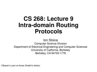
CS 268: Lecture 8Intra-domain Routing Protocols Scott Shenker and Ion Stoica Computer Science Division Department of Electrical Engineering and Computer Sciences University of California, Berkeley Berkeley, CA 94720-1776 (*Based in part on Aman Shaikh’s slides)
Internet Routing • Internet organized as a two level hierarchy • First level – autonomous systems (AS’s) • AS – region of network under a single administrative domain • AS’s run an intra-domain routing protocols • Distance Vector, e.g., Routing Information Protocol (RIP) • Link State, e.g., Open Shortest Path First (OSPF) • Between AS’s runs inter-domain routing protocols, e.g., Border Gateway Routing (BGP) • De facto standard today, BGP-4
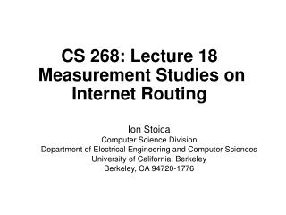
Example Interior router BGP router AS-1 AS-3 AS-2
Intra-domain Routing Protocols • Based on unreliable datagram delivery • Distance vector • Routing Information Protocol (RIP), based on Bellman-Ford • Each neighbor periodically exchange reachability information to its neighbors • Link state • Open Shortest Path First (OSPF), based on Dijkstra • Each network periodically floods immediate reachability information to other routers
5 3 5 2 2 1 3 1 2 1 C D B A E F Routing • Goal: determine a “good” path through the network from source to destination • Good means usually the shortest path • Network modeled as a graph • Routers nodes • Link edges • Edge cost: delay, congestion level,…
5 3 5 2 2 1 3 1 2 1 C D B A E F Routing Problem • Assume • A network with N nodes, where each edge is associated a cost • A node knows only its neighbors and the cost to reach them • How does each node learns how to reach every other node along the shortest path?
Host C Host D Host A N2 N1 N3 N5 Host B Host E N4 N6 N7 Distance Vector: Control Traffic • When the routing table of a node changes, the node sends its table to its neighbors • A node updates its table with information received from its neighbors
C D B A Example: Distance Vector Algorithm Node A Node B 3 2 1 1 7 Node C Node D 1 Initialization: 2 for all neighbors V do 3 ifV adjacent to A 4 D(A, V) = c(A,V); 5 else 6 D(A, V) = ∞; …
C D B A (D(C,A), D(C,B), D(C,D)) Example: 1st Iteration (C A) Node A Node B 3 2 1 1 7 … 7 loop: … 12 else if (update D(V, Y) received from V) 13 for all destinations Y do 14 if (destination Y through V) 15 D(A,Y) = D(A,V) + D(V, Y); 16 else 17 D(A, Y) = min(D(A, Y), D(A, V) + D(V, Y)); 18 if (there is a new minimum for dest. Y) 19 send D(A, Y) to all neighbors 20 forever Node C Node D
D(A, D) = min(D(A, D), D(A, C) + D(C,D) = min(∞ , 7 + 1) = 8 D C B A Example: 1st Iteration (C A) Node A Node B 3 2 1 1 7 … 7 loop: … 12 else if (update D(V, Y) received from V) 13 for all destinations Y do 14 if (destination Y through V) 15 D(A,Y) = D(A,V) + D(V, Y); 16 else 17 D(A, Y) = min(D(A, Y), D(A, V) + D(V, Y)); 18 if (there is a new minimum for dest. Y) 19 send D(A, Y) to all neighbors 20 forever (D(C,A), D(C,B), D(C,D)) Node C Node D
C D B A Example: 1st Iteration (C A) Node A Node B 3 2 1 1 7 … 7 loop: … 12 else if (update D(V, Y) received from V) 13 for all destinations Y do 14 if (destination Y through V) 15 D(A,Y) = D(A,V) + D(V, Y); 16 else 17 D(A, Y) = min(D(A, Y), D(A, V) + D(V, Y)); 18 if (there is a new minimum for dest. Y) 19 send D(A, Y) to all neighbors 20 forever Node C Node D
D(A,D) = min(D(A,D), D(A,B) + D(B,D)) = min(8, 2 + 3) = 5 D(A,C) = min(D(A,C), D(A,B) + D(B,C)) = min(7, 2 + 1) = 3 D C B A Example: 1st Iteration (BA, CA) Node A Node B 3 2 1 1 7 … 7 loop: … 12 else if (update D(V, Y) received from V) 13 for all destinations Y do 14 if (destination Y through V) 15 D(A,Y) = D(A,V) + D(V, Y); 16 else 17 D(A, Y) = min(D(A, Y), D(A, V) + D(V, Y)); 18 if (there is a new minimum for dest. Y) 19 send D(A, Y) to all neighbors 20 forever Node C Node D
C D B A Example: End of 1st Iteration Node A Node B 3 2 1 1 7 … 7 loop: … 12 else if (update D(V, Y) received from V) 13 for all destinations Y do 14 if (destination Y through V) 15 D(A,Y) = D(A,V) + D(V, Y); 16 else 17 D(A, Y) = min(D(A, Y), D(A, V) + D(V, Y)); 18 if (there is a new minimum for dest. Y) 19 send D(A, Y) to all neighbors 20 forever Node C Node D
C D B A Example: End of 3nd Iteration Node A Node B 3 2 1 1 7 … 7 loop: … 12 else if (update D(V, Y) received from V) 13 for all destinations Y do 14 if (destination Y through V) 15 D(A,Y) = D(A,V) + D(V, Y); 16 else 17 D(A, Y) = min(D(A, Y), D(A, V) + D(V, Y)); 18 if (there is a new minimum for dest. Y) 19 send D(A, Y) to all neighbors 20 forever Node C Node D Nothing changes algorithm terminates
1 4 1 50 C A B Distance Vector: Link Cost Changes 7 loop: 8 wait (link cost update or update message) 9 if (c(A,V) changes by d) 10 for all destinations Y through Vdo 11 D(A,Y) = D(A,Y) + d 12 else if (update D(V, Y) received from V) 13 for all destinations Y do 14 if (destination Y through V) 15 D(A,Y) = D(A,V) + D(V, Y); 16 else 17 D(A, Y) = min(D(A, Y), D(A, V) + D(V, Y)); 18 if (there is a new minimum for destination Y) 19 send D(A, Y) to all neighbors 20 forever “good news travels fast” Node B Node C time Link cost changes here Algorithm terminates
60 4 1 50 C A B Distance Vector: Count to Infinity Problem 7 loop: 8 wait (link cost update or update message) 9 if (c(A,V) changes by d) 10 for all destinations Y through Vdo 11 D(A,Y) = D(A,Y) + d 12 else if (update D(V, Y) received from V) 13 for all destinations Y do 14 if (destination Y through V) 15 D(A,Y) = D(A,V) + D(V, Y); 16 else 17 D(A, Y) = min(D(A, Y), D(A, V) + D(V, Y)); 18 if (there is a new minimum for destination Y) 19 send D(A, Y) to all neighbors 20 forever Node B “bad news travels slowly” Node C … time Link cost changes here; recall from slide 24 that B also maintains shortest distance to A through C, which is 6. Thus D(B, A) becomes 6 !
60 4 1 50 C A B Distance Vector: Poisoned Reverse • If C routes through B to get to A: • C tells B its (C’s) distance to A is infinite (so B won’t route to A via C) • Will this completely solve count to infinity problem? Node B Node C time Link cost changes here; B updates D(B, A) = 60 as C has advertised D(C, A) = ∞ Algorithm terminates
Host C Host D Host A N2 N1 N3 N5 Host B Host E N4 N6 N7 Link State: Control Traffic • Each node floods its local information to every other node in the network • Each node ends up knowing the entire network topology use Dijkstra to compute the shortest path to every other node
C C C C C C C A A A A A A A D D D D D D D Host C Host D Host A B B B B B B B E E E E E E E N2 N1 N3 N5 Host B Host E N4 N6 N7 Link State: Node State
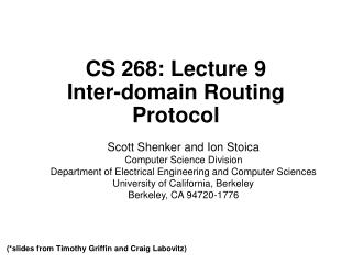
C D E A B F Example: Dijkstra’s Algorithm D(B),p(B) 2,A D(D),p(D) 1,A D(C),p(C) 5,A D(E),p(E) Step 0 1 2 3 4 5 start S A D(F),p(F) 1 Initialization: 2 S = {A}; 3 for all nodes v 4 if v adjacent to A 5 then D(v) = c(A,v); 6 else D(v) = ; … 5 3 5 2 2 1 3 1 2 1
C D E A B F Example: Dijkstra’s Algorithm D(B),p(B) 2,A D(D),p(D) 1,A D(C),p(C) 5,A 4,D D(E),p(E) 2,D Step 0 1 2 3 4 5 start S A AD D(F),p(F) • … • 8 Loop • 9 find w not in S s.t. D(w) is a minimum; • 10 add w to S; • update D(v) for all v adjacent • to w and not in S: • 12 D(v) = min( D(v), D(w) + c(w,v) ); • 13 until all nodes in S; 5 3 5 2 2 1 3 1 2 1
C D E A B F Example: Dijkstra’s Algorithm D(B),p(B) 2,A D(D),p(D) 1,A D(C),p(C) 5,A 4,D 3,E D(E),p(E) 2,D Step 0 1 2 3 4 5 start S A AD ADE D(F),p(F) 4,E • … • 8 Loop • 9 find w not in S s.t. D(w) is a minimum; • 10 add w to S; • update D(v) for all v adjacent • to w and not in S: • 12 D(v) = min( D(v), D(w) + c(w,v) ); • 13 until all nodes in S; 5 3 5 2 2 1 3 1 2 1
C D E A B F Example: Dijkstra’s Algorithm D(B),p(B) 2,A D(D),p(D) 1,A D(C),p(C) 5,A 4,D 3,E D(E),p(E) 2,D Step 0 1 2 3 4 5 start S A AD ADE ADEB D(F),p(F) 4,E • … • 8 Loop • 9 find w not in S s.t. D(w) is a minimum; • 10 add w to S; • update D(v) for all v adjacent • to w and not in S: • 12 D(v) = min( D(v), D(w) + c(w,v) ); • 13 until all nodes in S; 5 3 5 2 2 1 3 1 2 1
C D E A B F Example: Dijkstra’s Algorithm D(B),p(B) 2,A D(D),p(D) 1,A D(C),p(C) 5,A 4,D 3,E D(E),p(E) 2,D Step 0 1 2 3 4 5 start S A AD ADE ADEB ADEBC D(F),p(F) 4,E • … • 8 Loop • 9 find w not in S s.t. D(w) is a minimum; • 10 add w to S; • update D(v) for all v adjacent • to w and not in S: • 12 D(v) = min( D(v), D(w) + c(w,v) ); • 13 until all nodes in S; 5 3 5 2 2 1 3 1 2 1
C D E A B F Example: Dijkstra’s Algorithm D(B),p(B) 2,A D(D),p(D) 1,A D(C),p(C) 5,A 4,D 3,E D(E),p(E) 2,D Step 0 1 2 3 4 5 start S A AD ADE ADEB ADEBC ADEBCF D(F),p(F) 4,E • … • 8 Loop • 9 find w not in S s.t. D(w) is a minimum; • 10 add w to S; • update D(v) for all v adjacent • to w and not in S: • 12 D(v) = min( D(v), D(w) + c(w,v) ); • 13 until all nodes in S; 5 3 5 2 2 1 3 1 2 1
Message complexity LS: O(n2*e) messages n: number of nodes e: number of edges DV: O(d*n*k) messages d: node’s degree k: number of rounds Time complexity LS: O(n*log n) DV: O(n) Convergence time LS: O(1) DV: O(k) Robustness: what happens if router malfunctions? LS: node can advertise incorrect link cost each node computes only its own table DV: node can advertise incorrect path cost each node’s table used by others; error propagate through network Link State vs. Distance Vector
Open Shortest Path First (OSPF) • All routers in the domain come to a consistent view of the topology by exchange of Link State Advertisements (LSAs) • Router describes its local connectivity (i.e., set of links) in an LSA • Set of LSAs (self-originated + received) at a router = topology • Hierarchical routing • OSPF domain can be divided into areas • Hub-and-spoke topology with area 0 as hub and other non-zero areas as spokes
OSPF Performance • OSPF processing impacts convergence, (in)stability • Load is increasing as networks grow • Bulk of OSPF processing is due to LSAs • Sending/receiving LSAs • LSAs can trigger Route calculation (Dijkstra’s algorithm) • Understanding dynamics of LSA traffic is key for a better understanding of OSPF
Objectives for OSPF Monitor • Real-time analysis of OSPF behavior • Trouble-shooting, alerting, validation of maintenance • Real-time snapshots of OSPF network topology • Off-line analysis • Post-mortem analysis of recurring problems • Generate statistics and reports about network performance • Identify anomaly signatures • Facilitate tuning of configurable parameters • Analyze OSPF behavior in commercial networks
Categorizing LSA Traffic Change LSAs • A router originates an LSA due to… • Change in network topology • Example: link goes down or comes up • Detection of anomalies and problems • Periodic soft-state refresh • Recommended value of interval is 30 minutes • Forms baseline LSA traffic • LSAs are disseminated using reliable flooding • Includes change and refresh LSAs • Flooding leads to duplicate copies of LSAs being received at a router • Overhead: wastes resources Refresh LSAs Duplicate LSAs
Components • Data collection: LSA Reflector (LSAR) • Passively collects OSPF LSAs from network • “Reflects” streams of LSAs to LSAG • Archives LSAs for analysis by OSPFScan • Real-time analysis: LSA aGgregator (LSAG) • Monitors network for topology changes, LSA storms, node flaps and anomalies • Off-line analysis: OSPFScan • Supports queries on LSA archives • Allows playback and modeling of topology changes • Allows emulation of OSPF routing
LSAG Real-time Monitoring OSPFScan Off-line Analysis LSA archive LSA archive LSA archive Example LSAs LSAs TCP Connection LSAs LSAR 1 LSAR 2 “Reflect” LSA “Reflect” LSA replicate LSAs LSAs LSAs OSPF Network Area 0 Area 2 Area 1
How LSAR attaches to Network • Host mode: Join multicast group • Full adjacency mode: form full adjacency (= peering session) with a router • Partial adjacency mode: keep adjacency in a state that allows LSAR to receive LSAs, but does not allow data forwarding over link
How LSAR attaches to Network • Host mode • Join multicast group • Adv: completely passive • Disadv: not reliable, delayed initialization of LSDB • Full adjacency mode • Form full adjacency (= peering session) with a router • Adv: reliable, immediate initialization of LSDB • Disadv: LSAR’s instability can impact entire network • Partial adjacency mode • Keep adjacency in a state that allows LSAR to receive LSAs, but does not allow data forwarding over link • Adv: reliable, LSAR’s instability does not impact entire network, immediate initialization of LSDB • Disadv: can raise alarms on the router
LSAR R Please send me LSA L Please send me LSA L Please send me LSA L I have LSA L Partial Adjacency for LSAR I need LSA L from LSAR Partial state • Router R does not advertise a link to LSAR • LSAR does not originate any LSAs • Routers (except R) not aware of LSAR’s presence • Does not trigger routing calculations in network • LSAR’s going up/down does not impact network • LSARR link is not used for data forwarding
Performance Evaluation • Performance of LSAR and LSAG through lab experiments • LSAR and LSAG are key to real-time monitoring • How performance scales with LSA-rate and network size
Measure LSA processing time for LSAG LSA LSA LSA Emulated topology LSA LSA Measure LSA pass-through time for LSAR Experimental Setup PC SUT LSAG TCP connection OSPF adjacency Zebra LSAR TCP connection
Methodology • Send a burst of LSAs from Zebra to LSAR • Vary number of LSAs (l) in a burst of 1 sec duration • Use of fully connected graph as the emulated topology • Vary number of nodes (n) in the topology • Performance measurements • LSAR performance: LSA “pass-through” time • Zebra measures time difference between sending and receiving an LSA from LSAR • LSAG performance: LSA processing time • Instrumentation of LSAG code
Enterprise Network Case Study • The network provides customers with connectivity to applications and databases residing in the data center • OSPF network • 15 areas, 500 routers • This case study covers 8 areas, 250 routers • One month: April 2002 • Link-layer = Ethernet-based LANs • Customers are connected via leased lines • Customer routes are injected via EIGRP into OSPF • The routes are propagated via external LSAs • Quite reasonable for the enterprise network in question
External (EIGRP) Area A LAN1 LAN2 B1 B2 Monitor Border rtrs Area 0 Enterprise Network Topology Customer Customer Customer OSPF Domain Area A Area B Area 0 Area C Monitor is completely passive No adjacencies with any routers Receives LSAs on a multicast group Servers Database Applications
Highlights of the Results • Categorize, baseline and predict • Categories: Refresh, Change, Duplicate; External, Internal • Bulk of LSA traffic is due to refresh • Refresh LSA traffic is smooth: no evidence of refresh synchronization across network • Refresh LSA traffic is predictable from router configuration info • Detect, diagnose and act • Almost all LSAs arise from persistent yet partial failure modes • Internal LSA spikes • Indicate router hardware degradation • Carry out preventive maintenance • External LSA spikes • Indicate degradation in customer connectivity • Call customer before customer calls you • Propose Improvements • Simple configuration changes to reduce duplicate LSA traffic
Area 0 Area 2 Genuine Anomaly Genuine Anomaly Days Days Artifact: 23 hr day (Apr 7) Days Days Area 3 Area 4 LSA Traffic in Different Areas Refresh LSAs Change LSAs Duplicate LSAs
Baseline LSA Traffic: Refresh LSAs • Refresh LSA traffic can be reliably predicted using information available in router configuration files • Important for workload modeling • See paper for details Days Days Area 2 Area 3
Refresh process is not synchronized Negligible LSA clumping • No evidence of synchronization • Contrary to simulation-based study in [Basu01] • Reasons • Changes in the topology help break synchronization • LSA refresh at one router is not coupled with LSA refresh at other routers • Drift in the refresh interval of different routers
Anomaly Detection: Change LSAs Days • Internal to OSPF domain versus external • Change LSAs due to external events dominated • Not surprising due to large number of leased lines used to import customer routes into OSPF • Customer volatility network volatility
Root Causes of Change LSAs • Persistent problem flapping numerous change LSAs • Internal LSA spikes hardware router problems • OSPF monitor identified a problem early and led to preventive maintenance • External LSA spikes customer route volatility • Overload of an external link to a customer between 8 pm – 4 am causes EIGRP session on that link to flap
Overhead: Duplicate LSAs • Why do some areas witness substantial duplicate LSA traffic, while other areas do not witness any? • OSPF flooding over LANs leads to control plane asymmetries and to imbalances in duplicate LSA traffic Days
DR BDR OSPF Operations over Broadcast Networks • Each node sends an LSA to multicast group DR-rtrs • Both designated router (DR) and backup designated router BDR subscribe to this group • DR floods the LSA back to all routers on the network • Send to all-rtrs multicast group to which all nodes subscribe DR BDR