Download
1 / 18
220 likes | 489 Views
Pulse Code Modulation. Pulse Code Modulation Analogue to Digital Conversion Quantizing Encoding. Pulse Code Modulation.

E N D
Pulse Code Modulation Pulse Code Modulation Analogue to Digital Conversion Quantizing Encoding
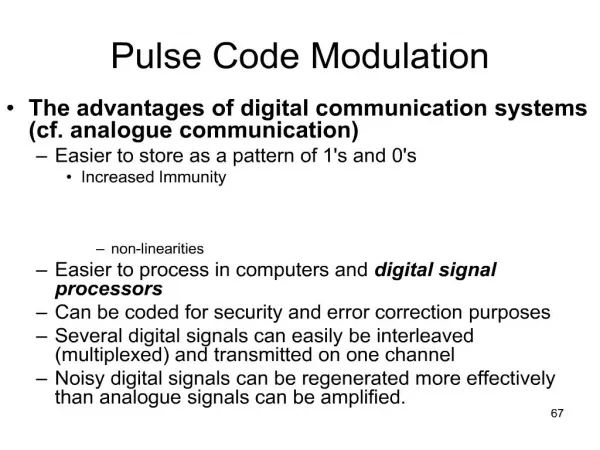
Pulse Code Modulation DEFINITION: Pulse code modulation (PCM) is essentially analog-to-digital conversion of a special type where the information contained in the instantaneous samples of an analog signal is represented by digital words in a serial bit stream. The advantages of PCM are: Relatively inexpensive digital circuitry may be used extensively. PCM signals derived from all types of analog sources may be merged with data signals and transmitted over a common high-speed digital communication system. In long-distance digital telephone systems requiring repeaters, a clean PCM waveform can be regenerated at the output of each repeater, where the input consists of a noisy PCM waveform. The noise performance of a digital system can be superior to that of an analog system. The probability of error for the system output can be reduced even further by the use of appropriate coding techniques.
Sampling, Quantizing, and Encoding • The PCM signal is generated by carrying out three basic operations: • Sampling • Quantizing • Encoding • Sampling operation generates a flat-top PAM signal. • Quantizing operation approximates the analog values by using a finite number of levels. This operation is considered in 3 steps • Uniform Quantizer • Quantization Error • Quantized PAM signal output • PCM signal is obtained from the quantized PAM signal by encoding each quantized sample value into a digital word.
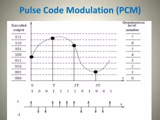
111 110 101 100 011 010 001 000 Digital Output Signal 111 111 001 010 011 111 011 Analog Input Signal Sample Analog to Digital Conversion ADC Quantize Encode The Analog-to-digital Converter (ADC) performs three functions: Sampling Makes the signal discrete in time. If the analog input has a bandwidth of W Hz, then the minimum sample frequency such that the signal can be reconstructed without distortion. Quantization Makes the signal discrete in amplitude. Round off to one of q discrete levels. Encode Maps the quantized values to digital words that are bits long. If the (Nyquist) Sampling Theorem is satisfied, then only quantization introduces distortion to the system.
Uniform Quantization • Most ADC’s use uniform quantizers. • The quantization levels of a uniform quantizer are equally spaced apart. • Uniform quantizers are optimal when the input distribution is uniform. When all values within the Dynamic Range of the quantizer are equally likely.
Quantization Example Analogue signal Sampling TIMING Quantization levels. Quantized to 5-levels Quantization levels Quantized 10-levels
QUANTIZATION The used of a non-uniform quantizer is equivalent to passing the baseband Signal through a compressor and then appling the compressed signal to a uniform quantizer. A particular form of compression law that used in practice is the so-called μ-law is defined by
Encoding • The output of the quantizer is one of M possible signal levels. • If we want to use a binary transmission system, then we need to map each quantized sample into an n bit binary word. • Encoding is the process of representing each quantized sample by an bit code word. • The mapping is one-to-one so there is no distortion introduced by encoding. • Some mappings are better than others. • A Gray code gives the best end-to-end performance. • The weakness of Gray codes is poor performance when the sign bit (MSB) is received in error.
Gray Codes • With gray codes adjacent samples differ only in one bit position. • Example (3 bit quantization): XQ Natural coding Gray Coding +7 111 110 +5 110 111 +3 101 101 +1 100 100 -1 011 000 -3 010 001 -5 001 011 -7 000 010 • With this gray code, a single bit error will result in an amplitude error of only 2. • Unless the MSB is in error.
PCM encoding example Levels are encoded using this table Table: Quantization levels with belonging code words Chart 2. Process of restoring a signal. PCM encoded signal in binary form: 101 111 110 001 010 100 111 100 011 010 101 Total of 33 bits were used to encode a signal Chart 1. Quantization and digitalization of a signal. Signal is quantized in 11 time points & 8 quantization segments.