Download
1 / 31
310 likes | 312 Views
This lecture discusses the effects of atmospheric turbulence on telescope resolution and the use of adaptive optics to correct for wavefront distortions. It also explores the principles of interferometry and its applications in high-resolution imaging. Topics include the use of laser guide stars, Strehl ratio as a measure of performance, multi-conjugate adaptive optics, and space interferometry missions.

E N D
ASTRO 2233 Fall 2010 Adaptive Optics, Interferometry and Planet Detection Lecture 16 Thursday October 21, 2010
Projects: Everyone has submitted an outline. After reading the Astro2010 reports and additional class discussions you can change topics if you wish but discuss it with me. Next Tuesday: Phil Muirhead
Effects of Atmospheric Turbulence on “Seeing” – i.e. telescope effective resolution SOLUTION – ADAPTIVE OPTICS (AO) Refractive index of atmosphere at 0.5 m n = 1 + 79 x 10-6 P / T ; P (ressure) in millibars T(emperature) in Kelvin = 1.0003 for P = 1,000 mBar; T = 300K Variations due to small fluctuations in T (and P)
Adaptive Optics Ref: Center for Adaptive Optics Wavefront sensor See http://www.ucolick.org/~max/289C/ lecture 6 - Claire Max, Center for Adaptive Optics
Correcting the wavefront using tilt information from the wavefront sensor Claire Max, Center for Adaptive Optics
How often do you need to correct wavefront? How fast does the atmosphere change? - depends on wind speed at turbulent layer Time constant for an isoplanetic patch size of 20 cm = 0.31 20/Vavg Vavg is average wind speed For Vavg = 20 m/s (70 km/hr) Time constant = 3 ms - need to correct wavefront every 1 ms In the near infra-red where patch size is ~1 m Time constant ~ 15 ms - need to correct wavefront ~100 times/sec Much easier in the near infra-red - slower correction - fewer actuators due to larger patch size
LASER GUIDE “STARS” Path of laser on Gemini North. The laser is located at the bottom of the yellow/orange beam near the right middle of the image. Note that the laser's light is directed by "relay optics" that direct the light to a "launch telescope" located behind the secondary mirror at the top/center of the telescope. Illustration based on Gemini computer animation. Laser reflects off sodium layer at ~80 km altitude (a) Astronomers using Keck’s adaptive optics have obtained the best pictures yet of the planet Neptune. The images show bands encircling the planet and what appear to be fast-moving storms of haze. (b) The same image without adaptive optics (I. de Pater).
Measure of Performance – STREHL RATIO Measure of the optical quality of a telescope including “seeing” problems due to atmospheric turbulence Strehl Ratio = Ratio of the amplitude of the point spread function (PSF) – the diffraction pattern - with and without the atmosphere assuming a perfect telescope. Point spread function for no atmosphere – Strehl ratio = 1.0
Multi-conjugate adaptive optics– multiple guide stars - allows three dimensional reconstruction of atmospheric turbulence and wider fields of view (European Southern Observatory slide)
Extreme adaptive optics – high resolution and high contrast imaging • Multiple guide stars • Thousands of actuators on deformable mirror • Very high precision for setting deformable mirror - a few nm • Very high speed in setting deformable mirror – several kHz Center for Adaptive Optics image
INTERFEROMETRY - Very high resolution Angular separation of nulls in diffraction pattern = λ/d
INTERFEROMETRY k = 2 π/λ
VERY LARGE ARRAY Very Large Array, New Mexico
Atacama Large Millimeter Array Wavelengths 350 m to 1 cm Best resolution ~10 mas
RESOLUTION = λ/D VLA (A array) at 3.5 cm: Resolution ~ 0.2 arcsec Atacama mm array: Resolution ~ 0.02 arcsec at 1 mm wavelength
Keck 10-m optical telescopes, Hawaii. Experimental interferometer.
LARGE BINOCULAR TELESCOPE Mt Graham, Arizona Two 8.4 m mirrors spaced 14.4 m apart 8.4 m => ~14 mas resolution (no atmosphere) 14.4 m => 8 mas fringe spacing as interferometer
European Southern Observatory (ESO) Very Large Telescope(S) - 4 x 8M
Space Interferometry Mission - SIM What: Interferometer – 10m baseline Positional Accuracy – 4 μarcsec (1 μarcsec relative over 1 deg field) Distance measurements: 1% accuracy to several thousand parsecs 10% over whole galaxy CALIBRATE CEPHEID and RR LYRA VARIABLE STARS Planet search – astrometric search nulling interferometer tests dynamic range of 104
Detection of Angular Motion of the Parent Star about the Center-of-Mass of System • No periodic motion means no planet – or planet to small/distant from star • Astrometry – measuring the positional motion of the star • Remember for two bodies in a circular orbit about each other – i.e. about the CM: • m1 r1 =m2 r2 • For a planet about a star • a☼ = mpap / m☼- what is this telling us about the radius of the orbit • of a planet that would make it easiest to detect • where a☼ = radius of star orbit via periodic positional changes of the star? • ap= radius of planet orbit – large is good => bigger star orbit radius • The angular shift in the star’s position is : • θ = a☼ / R radians where R is the distance to the star from Earth • = {mpap / m☼} / R arc sec if ap is in AU and R is in parsecs
ASTROMETRY – measuring angular deflection of the parent star about center of mass of system Sun’s trajectory about the center-of-mass of the solar system. As viewed from 10 parsecs (32 light years) away.
2. Velocity of the Star measurements via Doppler Shift Example: for circular orbits, planet-star pair, * = velocity of star p is the orbit period r1 = radius of star orbit about center-of-mass = a m2/(m1 + m2) a = star-planet distance from Keppler’s 3rd law, a3 p2 For Circular Orbit Basis for discovering extra-solar planets Maximum velocity for elliptical orbits http://upload.wikimedia.org/wikipedia/commons/5/59/Orbit3.gif
For a star in a circular orbit and assuming that mp << m☼ then: The measured maximum velocity is given by vmax = 28.4 p-1/3 {mp Sin i / MJ} m☼-2/3 m sec-1 Where p is the orbit period in years, Sin i is the sine of the orbit inclination relative to the line-of-sight from Earth, MJ is the mass of Jupiter and m☼ is the mass of the star in solar masses. For an elliptical orbit: vmax = {2 G / p}1/3 {mp Sin i / (mp + m☼)2/3} {1 / (1 – e2)1/2} m sec-1 Jupiter orbiting the Sun: vmax = 12.5 m sec-1, where p = 11.9 years For Earth orbiting the Sun vmax = 0.1 m sec-1 - very difficult to measure
The measured maximum velocity is given by vmax = 28.4 p-1/3 {mp Sin i / MJ} m☼-2/3 m sec-1 Where p is the orbit period in years, Sin i is the sine of the orbit inclination relative to the line-of-sight from Earth, MJ is the mass of Jupiter and m☼ is the mass of the star in solar masses. Gliese 281 g: m☼ = 0.3 solar masses P = 36.5 days = 0.1 years Sin i = 1 mp = 3 Earth masses = 0.01 mass of Jupiter Velocity = 1.36 m/sec
Astrometry: Advantages: Direct measurement of mass of the planet – assumes we know star’s mass from stellar type – i.e. spectral class Sensitive to large planets a long way from the star Disadvantages: θ 1 / Distance to the star => nearby stars only [θmax for Sun – Jupiter from 10 light years 1.6 milli arc sec] Velocity measurements: Advantages: Sensitive to large planets close to the star Not directly dependent on distance to the star – just need sensitivity Disadvantages: mp Sin i - lower limit on the mass Not sensitive to planets at large distances from the star