Download

1 / 22
220 likes | 430 Views
This guy is wearing a haircut called a “Mullet”. Lecture 19 Unsupervised and One-Shot Learning. Gary Bradski and Sebastian Thrun. http://robots.stanford.edu/cs223b/index.html. Find the Mullets…. One-Shot Learning. One-Shot Learning.

E N D
This guy is wearing a haircut called a “Mullet” Lecture 19Unsupervised and One-Shot Learning Gary Bradski and Sebastian Thrun http://robots.stanford.edu/cs223b/index.html
Find the Mullets… One-Shot Learning
One-Shot Learning “The appearance of the categories we know and … the variability in their appearance, gives us important information on what to expect in a new category”1 Papers for this lecture: • L. Fei-Fei, R. Fergus and P. Perona, “A Bayesian Approach to Unsupervised One-Shot Learning of Object Categories” ICCV 03. • R. Fergus, P. Perona and A.Zisserman, “Object Class Recognition by Unsupervised Scale-Invariant Learning”, CVPR 03. • http://www.vision.caltech.edu/html-files/publications.html
…But first, review: Problem: • You have atleast 8 points (say, found with SIFT features) that you’ve tracked between 2 frames of a moving camera. • What are their 3D coordinates (up to a scale factor) relative to the first frame’s coordinate system? Answer: • Trucco, Ch. 7 Section 7.3.3-7.3.5, 7.4.2
P Pl Pr Yr p p r l Yl Zl Zr Xl fl fr Ol Or R, T Xr 2 Images • Notations • Pl =(Xl, Yl, Zl), Pr =(Xr, Yr, Zr) • Vectors of the same 3-D point P, in the left and right camera coordinate systems respectively • Extrinsic Parameters • Translation Vector T = (Or-Ol) • Rotation Matrix R • pl =(xl, yl, zl), pr =(xr, yr, zr) • Projections of P on the left and right image plane respectively • For all image points, we have zl=fl, zr=fr From: Zhigang Zhu, NAC 8/203A http://www-cs.engr.ccny.cuny.edu/~zhu/VisionCourse-I6716.html
Fundamental Matrix • Mapping between points and epipolar lines in the pixel coordinate systems • With no prior knowledge on the stereo system • From Camera to Pixels: Matrices of intrinsic parameters • Parameters: • focal lengths x & y: fx, fy, • center of projection: ox, oy ? Rank (Mint) =3 Essential Matrix For one camera moving, Mr = Ml. From: Zhigang Zhu, NAC 8/203A http://www-cs.engr.ccny.cuny.edu/~zhu/VisionCourse-I6716.html
Fundamental Matrix Essential Matrix • Fundamental Matrix • Rank (F) = 2 • Encodes info on both intrinsic and extrinsic parameters • Enables full reconstruction of the epipolar geometry • In pixel coordinate systems without any knowledge of the intrinsic and extrinsic parameters • Linear equation of the 9 entries of F From: Zhigang Zhu, NAC 8/203A http://www-cs.engr.ccny.cuny.edu/~zhu/VisionCourse-I6716.html
Computing F: The Eight-point Algorithm • Input: n point correspondences ( n >= 8) • Construct homogeneous system Ax= 0 from • x = (f11,f12, ,f13, f21,f22,f23 f31,f32, f33) : entries in F • Each correspondence give one equation • A is a nx9 matrix • Obtain estimate F^ by SVD of A • x (up to a scale) is column of V corresponding to the least singular value • Enforce singularity constraint: since Rank (F) = 2 • Compute SVD of F^ • Set the smallest singular value to 0: D -> D’ • Correct estimate of F : • Output: the estimate of the fundamental matrix, F’ • Similarly we can compute E given intrinsic parameters From: Zhigang Zhu, NAC 8/203A http://www-cs.engr.ccny.cuny.edu/~zhu/VisionCourse-I6716.html
Reconstruction up to a Scale Factor • Assumption and Problem Statement • Under the assumption that only intrinsic parameters and more than 8 point correspondences are given • Compute the 3-D location from their projections, pl and pr, as well as the extrinsic parameters • Solution • Compute the essential matrix E from at least 8 correspondences • Estimate T (up to a scale and a sign) from E (=RS) using the orthogonal constraint of R, and then R (see Trucco 7.4.2) • End up with four different estimates of the pair (T, R) • Reconstruct the depth of each point, and pick up the correct sign of R and T. • Results: reconstructed 3D points (up to a common scale); • The scale can be determined if distance of two points (in space) are known From: Zhigang Zhu, NAC 8/203A http://www-cs.engr.ccny.cuny.edu/~zhu/VisionCourse-I6716.html
Visual learning is inefficient Slide from Li Fei-Fei http://www.vision.caltech.edu/feifeili/Resume.htm
Slide from Li Fei-Fei http://www.vision.caltech.edu/feifeili/Resume.htm No wonder a huge amount of data is needed to train models… How do we get to more biological levels of performance?
Use a Bayesian Framework Training set Appearance Shape Appearance Training set Shape set to 1.0
Representation • Use a scale invariant, scale sensing feature keypoint detector (like the first steps of Lowe’s SIFT). From: Rob Fergus http://www.robots.ox.ac.uk/%7Efergus/
Features Keys • A direct appearance model is taken around each located key. This is then normalized by it’s detected scale to an 11x11 window. PCA further reduces these features. From: Rob Fergus http://www.robots.ox.ac.uk/%7Efergus/
Add Model Hyper-parameters What are hyper-parameters? Parameters that bias parameters. For instance if you wanted to learn the probability of a coin turning up heads or tails, it would be stupid to observe 1 “head” and conclude: “heads 100%, tails 0%. Instead, we use a bimodal distribution to draw our parameter beliefs from until we have enough data. Model Params Learn Then hype-params
Learning • Assume that an object instance is the only • consistent thing somewhere in a scene. • We don’t know where to start, so we use • the initial random parameters. • (M) We find the best (consistent across images) assignment given the params. • (E) We refit the feature detector params. and repeat until converged. • Note that there isn’t much consistency • This repeats until it converges at the most consistent assignment with maximized parameters across images. • Fit with E-M (this example is a 3 part model) • We start with the dual problem of what to fit and where to fit it. From: Rob Fergus http://www.robots.ox.ac.uk/%7Efergus/
Result: Unsupervised Learning Slide from Li Fei-Fei http://www.vision.caltech.edu/feifeili/Resume.htm
Recognition • Bayesian Decision based Feature detector results: The shape model. The mean location is indicated by the cross, with the ellipse showing the uncertainty in location. The number by each part is the probability of that part being present. From: Rob Fergus http://www.robots.ox.ac.uk/%7Efergus/ Recognition Result: The appearance model closest to the mean of the appearance density of each part
Data Slide from Li Fei-Fei http://www.vision.caltech.edu/feifeili/Resume.htm 3 categories are trained extensively, the first is learned in 1-5 presentations. This is possible since E-M also trains the hyper-parameters which say what 3D models “look like”/where to look.
Results • One-Shot results: • Compare to batch approaches: From: Rob Fergus http://www.robots.ox.ac.uk/%7Efergus/
Using supervised classifiers for unsupervised learning. • Will discuss in class.