Download
1 / 66
680 likes | 861 Views
A NEW GEOMETRICAL INTERPRETATION OF THE LORENTZ TRANSFORM AND THE SPECIAL THEORY OF RELATIVITY. Lewis F. McIntyre, MS GRD, Inc. 6303 Little River Turnpike, Ste 320 Alexandria, VA 22312. AGENDA . PURPOSE BACKGROUND THE NEW GRAPHICAL APPROACH Lorentz Transform Relativistic Doppler

E N D
A NEW GEOMETRICAL INTERPRETATION OF THE LORENTZ TRANSFORM AND THE SPECIAL THEORY OF RELATIVITY Lewis F. McIntyre, MS GRD, Inc. 6303 Little River Turnpike, Ste 320 Alexandria, VA 22312
AGENDA • PURPOSE • BACKGROUND • THE NEW GRAPHICAL APPROACH • Lorentz Transform • Relativistic Doppler • Four-Vector Solutions • MASS, MOMENTUM & ENERGY
PURPOSE • DEVELOP A GRAPHICAL SOLUTION WHICH • Preserves Equal Units of Measure and Orthogonality in All Reference Frames • Can Accommodate Multiple Reference Frames • TO ASSIST STUDENTS IN GRASPING FUNDAMENTALS OF SPECIAL RELATIVITY
BACKGROUND • TRANSFORMATIONS • Galilean • Lorentz • THE MEASUREMENT & THE EVENT • REVIEW OF OTHER GRAPHICAL TECHNIQUES
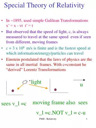
TRANSFORMATIONS RELATE A MEASUREMENT (x,y,z,t) OF AN EVENT IN ONE REFERENCE FRAME TO A MEASUREMENT (x*,y*, z*, t*) OF THAT SAME EVENT IN ANOTHER REFERENCE FRAME
The Galilean Transform • Parallel t and t* • Measurement of the Event e , and the Event, are Identical • c>>v t t* x*=x-vt y*=y t*=t x t=0 @ x=0 y* y vt x* e
The Lorentz Transform x t=T Y v= x/t t=T- t t x t=0 @ x=0
THE MEASUREMENT & THE EVENT • RADIAL DISTANCE IS INDETERMINATE! • INFERRING THE DISTANCE & TIME • Parallax • Active Interrogation • Simultaneous Solution of Lightline and Worldline
Determining Radial DistancePassive Measurement of Parallax PARALLAX AT ORIGINATOR PARALLAX AT OBSERVER OR RELATIVE BRIGHTNESS
Determining Radial DistanceActive Interrogation ctreturn x, ct cttransmission
Determining Radial DistanceSimultaneous Solution Between Lightline and Worldline ctreception cttransmission x=vt
REVIEW OF OTHER GRAPHICAL TECHNIQUES • THE MINKOWSKI SPACETIME DIAGRAM • TECHNIQUE • ADVANTAGES & DISADVANTAGES
Minkowski Spacetime Diagram 5 4.5 x* 4 t* 3.5 x* 3 2.5 Time t 2 1.5 1 x* 0.5 0 0 1 2 3 Distance x The Minkowski Space-time Diagram t* t* t*
Minkowski Spacetime Diagram 5 4.5 4 3.5 3 2.5 Time t 2 1.5 1 0.5 0 0 1 2 3 Distance x The Minkowski Space-time DiagramStep 1: Locate the Worldline x=vt t*
Minkowski Spacetime Diagram 5 4.5 4 t* 3.5 3 2.5 Time t 2 1.5 1 x* 0.5 0 0 1 2 3 Distance x The Minkowski Space-time DiagramErect the x* axis:t=xv
Minkowski Spacetime Diagram 5 4.5 4 t* 3.5 3 2.5 Time t 2 1.5 1 x* 0.5 0 0 1 2 3 Distance x The Minkowski Space-time DiagramErect Hyberbolic Lines of equal : t2=x2+ 2
Minkowski Spacetime Diagram 5 4.5 4 t* 3.5 3 2.5 Time t 2 1.5 1 x* 0.5 0 0 1 2 3 Distance x The Minkowski Space-time Diagram Erect Hyberbolic Lines of “Anti-”: t2=x2- 2
Minkowski Spacetime Diagram 5 4.5 4 t* 3.5 3 t* 2.5 Time t t* 2 t* 1.5 1 x* 0.5 0 0 1 2 3 Distance x The Minkowski Space-time Diagram Erect Lines of Equal t*
Minkowski Spacetime Diagram 5 4.5 x* 4 t* 3.5 x* 3 2.5 Time t 2 1.5 1 x* 0.5 0 0 1 2 3 Distance x The Minkowski Space-time Diagram Erect Lines of Equal x* t* t* t*
Minkowski Spacetime Diagram 5 4.5 The point indicated x=2.0, t=3.0 is read as x*=0.577, t*=2.308 4 t* 3.5 3 2.5 Time t 2 1.5 1 x* 0.5 0 0 1 2 3 Distance x The Minkowski Space-time Diagram One Event, Different Measurements
The Minkowski Space-time Diagram Advantages & Disadvantages • ADVANTAGES • Events And Measurements Are Identical • DISADVANTAGES • Only One Pair of Reference Frames • Unique Construction for Each Velocity • One Reference Frame Distorted • Units of Measure “Stretched” • Not Orthogonal
THE NEW GRAPHICAL APPROACH • LORENTZ TRANSFORM • Events on the Worldline • Doppler • The Generalized Lorentz Transform • FOUR-VECTOR SOLUTIONS • MASS, MOMENTUM & ENERGY
e O The Velocity TriangleAn Event on a Worldline timeline of S worldline of S* in S x=vt x3 ct3
A2 A3 O The Velocity TriangleThe Inferential Circle timeline of S worldline of S* in S ct2=ct3+x3 x3 ct3 A A1 ct1 =ct3-x3
A2 A3 O The Velocity TriangleLocate the Proper Time timeline of S worldline of S* in S x3 ct3 A A1
A2 A3 O The Velocity TriangleDetermine the Proper Time timeline of S worldline of S* in S x3 ct3 A A4 A1 (c)2= (ct3) 2 -x3 2 ct3*=c
A2 A3 A4 A O The Velocity TriangleThe Lorentz Angle timeline of S worldline of S* in S timeline of S* x3 ct3
A3 O Radial And Hyperbolic Tau Hyperbolic : A measurement x,t in S’s coordinates x3 ct3 A A4 Radial : Elapsed Proper Time since collocation c=ct3* radius c
A3 B3 O Same Tau, Different Velocities... B x3 ct3 A A4 B4 radius c
A3 B3 O …No Matter How Many! C C3 B x3 ct3 A A4 B4 C4 radius c
A2 A3 O Relativistic DopplerTime of Receipt from Proper Time of Event The Time of Receipt is Relativistically Doppler-Shifted from the Time of Transmission: Equal Units of Distance in the Plane of Origination to Equal Units of Time in the Plane of Receipt timeline of S worldline of S* in S ct2 x3 ct3 A ct*3 A4 A1 ct1
Relativistic Doppler Up and Down Doppler-Moving Source timeline of S worldline of S* in S DOWN-DOPPLER: Leaving Collocation, t>0 ct2 ct*3 UP-DOPPLER: Approaching Collocation, t<0 -ct*3
Relativistic Doppler Up and Down Doppler-Fixed Source timeline of S worldline of S* in S ct*3 ct2 -ct2
A2 A3 O Relativistic Doppler Time of Event from Time of Interrogation timeline of S worldline of S* in S ct2 The Product of Two Relativistic Doppler Shifts Yields a Classical Doppler Shift x3 ct3 A ct*3 A4 A1 ct1
A2 A3 A A4 O Relativistic Doppler Proper Time vs. Inferred Time timeline of S worldline of S* in S ct2 x3 ct3 A1 ct1
A2 A3 O Relativistic Doppler Proper Time of Transmission and Proper Time of Receipt timeline of S worldline of S* in S ct2 x3 ct3 A ct*3 A4 A1 ct1
A2 x3= (ct2-ct1)/2 ct3=(ct2+ct1)/2 A A3 A1 O Generalized Lorentz Transform A Measurement Not on the Worldline • S*’s Measurement Simultaneous with S’s at x3, t3 • Arrives at x3, t3 simultaneously with S*’s • Must start at ct’1 • Must end at ct’2 Timeline of S Worldline of S* in S timeline of S* ct2 ct’2 ct’1 ct1
A2 x3= (ct2-ct1)/2 ct3=(ct2+ct1)/2 A A3 A1 O Generalized Lorentz Transform Proper Times of S*’s Measurement Timeline of S Worldline of S* in S • S*’s Measurement Simultaneous with S’s at x3, t3 • Arrives at x3, t3 simultaneously with S*’s • Must start at ct’1 • Must end at ct’2 timeline of S* ct2 ct*2 ct*1 ct1
A2 x3= (ct2-ct1)/2 ct3=(ct2+ct1)/2 A A3 A1 O Generalized Lorentz Transform S*’s Measurement, Using the Same c Timeline of S Worldline of S* in S • S*’s Measurement Simultaneous with S’s at x3, t3 • Arrives at x3, t3 simultaneously with S*’s • Must start at ct’1 • Must end at ct’2 timeline of S* ct2 ct*2 A3* ct*1 ct1
Generalized Lorentz Transform Solving for x*, t* in Terms of x, t
Eddington’s Cigar • A SPACECRAFT FLIES BY EARTH AT 0.866C • AT FLY-BY, OBSERVERS ON EARTH AND IN THE SPACECRAFT BOTH LIGHT 30 MINUTE CIGARS • AT THE END OF THE SMOKE, EACH INFORMS THE OTHER OF THE EVENT • BOTH DETERMINE THAT THE OTHER’S CIGAR LASTED TWICE AS LONG
A1 B1 O Eddington’s Cigar Proper Duration of the Smokes
A2 A3 A1 B1 O Eddington’s Cigar A’s Receipt and Inference worldline of S* in S ct3, x3
B2 B3 A1 B1 O Eddington’s Cigar B’s Receipt and Inference worldline of S in S* ct*3, x*3
FOUR VECTOR SOLUTIONS • A SIMPLIFIED GRAPHICAL SOLUTION • THE DISPLACEMENT FOUR-VECTOR • THE VELOCITY FOUR-VECTOR
ct -0.707 -0.500 -0.266 0.0 0.266 0.500 0.707 0O -15O 15O 30O -30O 0.8 45O -45O 0.866 -0.866 0.6 -60O 60O 0.4 -0.966 0.966 -75O 75O 0.2 90O -90O -0.8 -0.6 -0.4 -0.2 0.2 0.4 0.6 0.8 x APPROACHING VELOCITIES RECEDING VELOCITIES APPROACHING VELOCITIES RECEDING VELOCITIES -0.2 105O -105O 0.966 -0.966 -0.4 -120O 120O -0.6 0.866 -0.866 -135O 135O -0.8 -150O 150O -165O 165O 180O 0.707 0.500 0.266 0.0 -0.500 -0.707 -0.266 THE WORKSHEET Velocity Preferred Frame Time Axis Lorentz Angle Preferred Frame x- Axis
ct -0.707 -0.500 -0.266 0.0 0.266 0.500 0.707 0O -15O 15O 30O -30O 0.8 A 45O -45O 0.866 -0.866 0.6 -60O 60O 0.4 -0.966 0.966 -75O 75O 0.2 90O -90O -0.8 -0.6 -0.4 -0.2 0.2 0.4 0.6 0.8 x APPROACHING VELOCITIES RECEDING VELOCITIES APPROACHING VELOCITIES RECEDING VELOCITIES -0.2 105O -105O 0.966 -0.966 Proper Time -0.4 S’s Measurement of S* -120O 120O S*’s Measurement of S -0.6 0.866 -0.866 -135O Intermediate Point 135O -0.8 -150O 150O -165O 165O 180O 0.707 0.500 0.266 0.0 -0.500 -0.707 -0.266 x=0.6 ct=0.8 THE SIMPLIFIED SOLUTION Locate thePoint Erect the Timeline x ct O
ct -0.707 -0.500 -0.266 0.0 0.266 0.500 0.707 0O -15O 15O 30O -30O 0.8 A 45O -45O 0.866 -0.866 0.6 A’ -60O 60O 0.4 -0.966 0.966 -75O 75O 0.2 90O -90O -0.8 -0.6 -0.4 -0.2 0.2 0.4 0.6 0.8 x APPROACHING VELOCITIES RECEDING VELOCITIES APPROACHING VELOCITIES RECEDING VELOCITIES -0.2 105O -105O 0.966 -0.966 Proper Time -0.4 S’s Measurement of S* -120O 120O S*’s Measurement of S -0.6 0.866 -0.866 -135O Intermediate Point 135O -0.8 -150O 150O -165O 165O 180O 0.707 0.500 0.266 0.0 -0.500 -0.707 -0.266 x=0.6 ct=0.8 THE SIMPLIFIED SOLUTION Erect the Intermediate Plane Locate the Intercept x ct Intermediate Plane: t*=t O