Download
1 / 13
160 likes | 404 Views
Lab 14 – Fall, 2012 Biaxial Interference Figures. Optical Mineralogy. Biaxial Sign: B x a Figures. To determine the optic sign of a biaxial mineral from a BX A figure, position the isogyres so that the melatopes are in the NE and SW quadrants

E N D
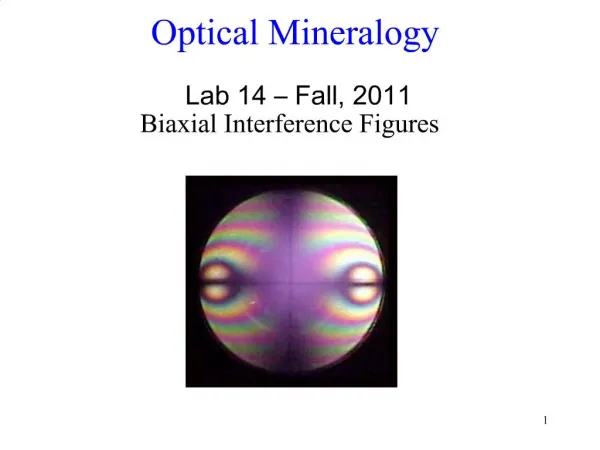
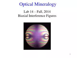
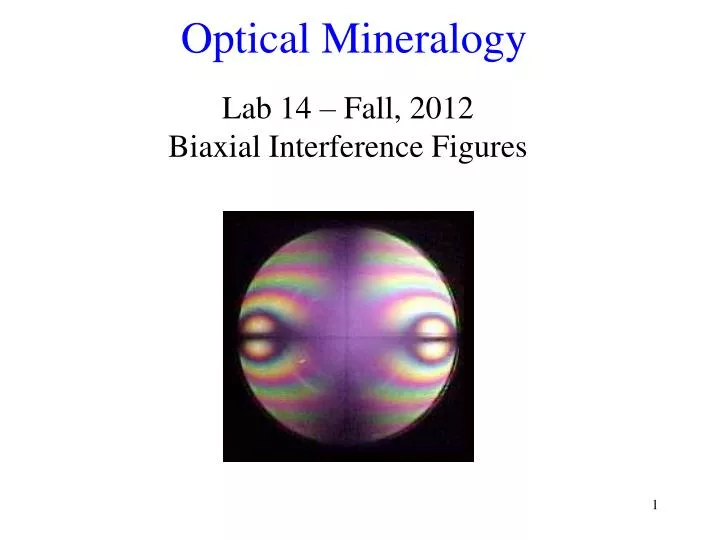
Lab 14 – Fall, 2012 Biaxial Interference Figures Optical Mineralogy
Biaxial Sign: Bxa Figures • To determine the optic sign of a biaxial mineral from a BXA figure, position the isogyres so that the melatopes are in the NE and SW quadrants • There should be an area near the melatopes that shows a 1o gray interference color • Observe this area as you insert the 550nm or 1o red compensator
Biaxial Sign: Bxa Figures • If the 1o gray area in region between the two isogyres turns yellow, the mineral is biaxial positive • If the 1o gray area inside of both the isogyres turns yellow the mineral is biaxial negative
Biaxial Sign: Centered OA Figures • Optic axis figures probably provide the easiest method for determination of optic sign because grains with an orientation that would produce an OA figure are perhaps the easiest to find • Place the isogyre so that the inside of the isogyre is in the NE quadrant • Find the area that shows 1o gray close to the melatope • Observe this area as the 550 nm compensator plate is inserted
Biaxial Sign: Centered OA Figures • If the area outside of the isogyre turns yellow, the mineral is biaxial positive • If the area inside the isogyre turns yellow, the mineral is biaxial negative
Biaxial Sign: Off-Centered Bxa or OA Figures • Probably even easier to locate are off-centered OA or BXA interference figures • Position the isogyre so that it fits best in either the NE or SW quadrant • Observe the gray area near the melatope and note the color change on insertion of the 550 nm compensator
Biaxial Sign: Off-Centered Bxa or OA Figures • If the gray area outside the isogyre turns yellow, the mineral is biaxial positive • If the gray area outside isogyre turns blue and the gray area inside the isogyre turns yellow, the mineral is biaxial negative
Estimation of 2V • Precise determination of 2V can only be made by determining the 3 principal refractive indices of the mineral • 2V can be estimated from Bxa and OA figures using the diagrams shown here
2V Estimation: Bxa Figure • For a BXA figure the distance between the melatopes is proportional to the 2V angle • To estimate the 2V from a BXA figure, it is necessary to know the numerical aperture (N.A.) of the objective lens used to observe the interference figure • The microscopes in our labs have an N.A. of between 0.65 and 0.85
2V Estimation: Bxa Figure • The diagram shown here gives a visual estimate of the 2V angle for objective lenses with these two values of N.A. for a mineral with a b refractive index of 1.6
2V Estimation: Bxa Figure • Remember that if the 2V is 0o the mineral is uniaxial, and would thus show the uniaxial interference figure • The separation of the isogyres or melatopes increases with 2V and the isogyres eventually go outside of the field of view for a 2V of 50o with the smaller N.A., and about 60o for the larger N.A
2V Estimation: Bxa Figure • Since the maximum 2V that can be observed for a Bxa figure depends on the b refractive index, the chart shown here may be useful to obtain more precise estimates if the b refractive index is known or can be measured As b increases, the maximum observable 2V decreases
2V Estimation: OAFigure • 2V estimates can be made on an optic axis figure by noting the curvature of the isogyres and referring to the diagram shown here • Note that the curvature is most for low values of 2V and decreases to where the isogyre essentially forms a straight line across the field of view for a 2V of 90o