Download

1 / 47
470 likes | 705 Views
Consortium for Comparative Genomics. University of Colorado School of Medicine. Multiple Sequence Alignment (MSA); short version BIOL 7711 Computational Bioscience. Sequence Alignment Profiles Mouse TCR V a. Why a Hidden Markov Model?.

E N D
Consortium for Comparative Genomics University of Colorado School of Medicine Multiple Sequence Alignment (MSA); short versionBIOL 7711 Computational Bioscience
Why a Hidden Markov Model? • Data elements are often linked by a string of connectivity, a linear sequence • Secondary structure prediction (Goldman, Thorne, Jones) • CpG islands • Models of exons, introns, regulatory regions, genes • Mutation rates along genome
Why a Hidden Markov Model? • Complications? • Insertion and deletion of states (indels) • Long-distance interactions • Benefits • Flexible probabilistic framework • E.g., compared to regular expressions
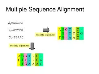
Multiple Sequence Alignment • Generalizepairwisealignment of sequences to include more than two • Looking at more than two sequences gives us much more information • Site-specific information • Sites are different! • E.g., which amino acids, coevolution • Process of change at a site • Evolutionary/phylogenetic relationships • Shorter branches, dissect compound indels
Sample MSA: cFOS FOS_RAT MMFSGFNADYEASSSRCSSASPAGDSLSYYHSPADSFSSMGSPVNTQDFCADLSVSSANF 60 FOS_MOUSE MMFSGFNADYEASSSRCSSASPAGDSLSYYHSPADSFSSMGSPVNTQDFCADLSVSSANF 60 FOS_CHICK MMYQGFAGEYEAPSSRCSSASPAGDSLTYYPSPADSFSSMGSPVNSQDFCTDLAVSSANF 60 FOSB_MOUSE -MFQAFPGDYDS-GSRCSS-SPSAESQ--YLSSVDSFGSPPTAAASQE-CAGLGEMPGSF 54 FOSB_HUMAN -MFQAFPGDYDS-GSRCSS-SPSAESQ--YLSSVDSFGSPPTAAASQE-CAGLGEMPGSF 54 *:..* .:*:: .***** **:.:* * *..***.* :.. :*: *:.*. ...* FOS_RAT IPTVTAISTSPDLQWLVQPTLVSSVAPSQ-------TRAPHPYGLPTPS-TGAYARAGVV 112 FOS_MOUSE IPTVTAISTSPDLQWLVQPTLVSSVAPSQ-------TRAPHPYGLPTQS-AGAYARAGMV 112 FOS_CHICK VPTVTAISTSPDLQWLVQPTLISSVAPSQ-------NRG-HPYGVPAPAPPAAYSRPAVL 112 FOSB_MOUSE VPTVTAITTSQDLQWLVQPTLISSMAQSQGQPLASQPPAVDPYDMPGTS----YSTPGLS 110 FOSB_HUMAN VPTVTAITTSQDLQWLVQPTLISSMAQSQGQPLASQPPVVDPYDMPGTS----YSTPGMS 110 :******:** **********:**:* **... ::. .**.:* : *: ..: FOS_RAT KTMSGGRAQSIG--------------------RRGKVEQLSPEEEEKRRIRRERNKMAAA 152 FOS_MOUSE KTVSGGRAQSIG--------------------RRGKVEQLSPEEEEKRRIRRERNKMAAA 152 FOS_CHICK KAP-GGRGQSIG--------------------RRGKVEQLSPEEEEKRRIRRERNKMAAA 151 FOSB_MOUSE AYSTGGASGSGGPSTSTTTSGPVSARPARARPRRPREETLTPEEEEKRRVRRERNKLAAA 170 FOSB_HUMAN GYSSGGASGSGGPSTSGTTSGPGPARPARARPRRPREETLTPEEEEKRRVRRERNKLAAA 170 :** . * *.::: :::.. .: .: : .** : * *:********:******:***
Optimal MSA • Use Dynamic Programming? • Optimal alignment algorithm exists, but is _________ • nis the number of sequences • L is the length of the longest sequence • 10 sequences of length 100 take 21010010~1023 operations, around 1 million years at 3GHz • Exponential algorithms strike again • So, approximation approaches?
Progressive MSA • Start with pairwise alignments of closely related sequences • Add more distantly related sequences one at a time • Complexity proportional to L2*n • Requiresa priori assumptions about the phylogenetic relationships • Can be estimated from all pairwisecomparisons • Unfortunate circularity to this approach • SATCHMO method tries to estimate both at once • MSA score based on sum of pairwise scores • Can be weighted to reduce influence of similar sequences
Gaps in Progressive MSAs • How to score gaps in MSAs? • Want to align gaps with each other over all sequences. A gap in a pairwise alignment that “matches” a gap in another pairwise alignment should cost less than introducing a totally new gap. • Possible that a new gap could be made to “match” an older one by shifting around the older pairwise alignment • Change gap penalty near conserved domains of various kinds (e.g. secondary structure, hydrophobic regions) • CLUSTALW2 http://www.ebi.ac.uk/Tools/clustalw2/is the most widely used Progressive MSA program
Greedy Algorithms • Best alignment of each new sequence to the existing alignment • Then never revisit the decision • Even if changing an old decision (e.g. moving around the gaps in a previous alignment) could increase the score, this approach doesn't do it. • Approach is called “greedy” because it uses the best solution at the current step, then moves on • Have to hope that the best solution to a part of the problem will be good solution for the whole problem • This is a common way to resolve exponential problems
Problems with Progressive MSA • Depends crucially on the quality of the pairwise alignments, particularly among the closest matches (which are aligned first) • Small errors propagate to whole alignment • There is no suitable resolution to the problem of gap penalties over multiple sequences • Works reasonably well for closely related sequences. • Even then, manual adjustments are common
Iterative MSA Methods • Start with a reasonable approximation to the optimal MSA • e.g. by using a progressive method • Then “tweak” to improve it • Common CS idea, called“optimization” • Various optimization techniques tried • e.g., GAs and simulated annealing • Key is the scoring function for the whole MSA • Also, what steps (tweaks) to take that are likely to improve the score
Block Based Methods • Start with short local alignments (blocks) • Then reduce the problem to aligning the regions between the blocks • “Divide and conquer” • Another common CS approach to exponential problems • How to find the blocks? • DALIGN (local alignment methods) • DCA (divide and conquer alignments) • Tmsa (identify patterns and use them to define blocks)
MSA Databases • E.g., Pfam, Tigergam, etc. • Look them up and surf
Protein motifs • Recall that local alignments can identify similar regions in non-homologous proteins • These regions (sometimes called domains) often have shared structure and/or function • Example: Zinc-finger DNA binding motif • How to define them? • Consensus sequence • Regular expression • Profile (probability for each amino acid at each position)
Recognizing ProSite patterns • L14 Ribosome pattern: [GA]-[LIV](3)-x(9,10)-[DNS]-G-x(4)-[FY]-x(2)-[NT]-x(2)-V-[LIV] • Some matching sequences: • GIIIACGHLIPQTNGACRTYILNDRVV • GVLLWQPKHCSNAADGAWAWFAATAAVL • ALIVEANIIILSISGRATTFHATSAVI • ProSite patterns can be translated into regular expressions, although the bounded length patterns (e.g. [LIV](3,5) are unwieldy to write down as regexps
Profiles • Rather than identifying only the “consensus” (i.e. most common) amino acid at a particular location, we can assign a probability to each amino acid in each position of the domain 1 2 3A 0.1 0.5 0.25C 0.3 0.1 0.25 D 0.2 0.2 0.25E 0.4 0.2 0.25
Applying a profile • Calculate score (probability of match) for a profile at each position in a sequence by multiplying individual probabilities. • Uses a “sliding window” • To calculate a significance value, normalize by the probability of match to random sequence 1 2 3A 0.1 0.5 0.25C 0.3 0.1 0.25 D 0.2 0.2 0.25E 0.4 0.2 0.25 For sequenceEACDC: EAC = .4 * .5 * .25 = .05ACD = .1 * .1 * .25 = .0025CDC = .3 * .2 * .25 = .015
Using motifs • Great for annotating a sequence with no strong homologs • INTERPRO is an uniform interface to many different motif methods and databases • ProSite • Prints (fingerprints = multiple motifs) • ProDom (like Pfam, but for domains) • SMART (mobile domains)
Creating profiles • Given a local MSA, creating a profile is straightforward • Calculate frequency of each amino acid at each position • What about zero frequencies? • Could be sampling errors, not real zero probabilities • Zero probabilities always make zero scores! • Regularization • Pseudocounts • Dirichlet mixtures (blend in background frequencies)
Better regularizers • Adding one pseudocountis too large and too uniform in the small MSA case • Instead, can add a fraction proportional to the overall frequency of occurrence of the amino acid • Might want to add different pseudocounts depending on the actual count (add more to smaller counts, especially 0) • Can use substitution matrices to estimate
Feature alphabets • Amino acids can be grouped by their characteristics: • Size, hydrophobicity, ionizability, etc. • An amino acid is generally in more than one group • Can set different regularizers (pseudocounts) for each different feature • Most useful when there are multiple features • otherwise many amino acids get same pseudocount
Dirichlet mixture priors • Fanciest (and near optimal) regularizer • Allows several dimensions (like a feature, but not predefined), each of which has a different weight for each amino acid. • Each pseudocount depends on the prior probability of seeing a particular distribution in a position • Add more “prior” to more unusual observations • Pseudocount falls off with more observations
A Simpler not very Hidden MMNucleotides, no Indels, Unambiguous Path G .1C .1A .7T .1 G .1C .3A .2T .4 G .3C .3A .1T .3 1.0 1.0 1.0 A 0.7 T 0.4 T 0.3
Emit G Emit C Begin End Emit A Emit T A Toy not-Hidden MMNucleotides, no Indels, Unambiguous PathAll arcs out are equal Example sequences:GATC ATC GC GAGAGC AGATTTC Arc Emission
A Simple HMMCpG Islands; States are Really Hidden Now 0.8 0.9 0.2 G .3C .3A .2T .2 G .1C .1A .4T .4 0.1 CpG Non-CpG
The Forward AlgorithmProbability of a Sequence is the Sum of All Paths that Can Produce It CpG 0.8 G .3C .3A .2T .2 G .3 .3*( .3*.8+ .1*.1) =.075 0.2 0.1 G .1 .1*( .3*.2+ .1*.9) =.015 G .1C .1A .4T .4 G C 0.9 Non-CpG
The Forward AlgorithmProbability of a Sequence is the Sum of All Paths that Can Produce It CpG 0.8 G .3C .3A .2T .2 G .3 .3*( .3*.8+ .1*.1) =.075 .3*( .075*.8+ .015*.1) =.0185 0.2 0.1 G .1 .1*( .3*.2+ .1*.9) =.015 .1*( .075*.2+ .015*.9) =.0029 G .1C .1A .4T .4 G C G 0.9 Non-CpG
The Forward AlgorithmProbability of a Sequence is the Sum of All Paths that Can Produce It CpG 0.8 G .3C .3A .2T .2 G .3 .3*( .3*.8+ .1*.1) =.075 .3*( .075*.8+ .015*.1) =.0185 .2*( .0185*.8+ .0029*.1) =.003 .2*( .003*.8+ .0025*.1) =.0005 0.2 0.1 G .1 .1*( .3*.2+ .1*.9) =.015 .1*( .075*.2+ .015*.9) =.0029 .4*( .0185*.2+ .0029*.9) =.0025 .4*( .003*.2+ .0025*.9) =.0011 G .1C .1A .4T .4 G C G A A 0.9 Non-CpG
The Forward AlgorithmProbability of a Sequence is the Sum of All Paths that Can Produce It CpG 0.8 G .3C .3A .2T .2 G .3 .3*( .3*.8+ .1*.1) =.075 .3*( .075*.8+ .015*.1) =.0185 .2*( .0185*.8+ .0029*.1) =.003 .2*( .003*.8+ .0025*.1) =.0005 0.2 0.1 G .1 .1*( .3*.2+ .1*.9) =.015 .1*( .075*.2+ .015*.9) =.0029 .4*( .0185*.2+ .0029*.9) =.0025 .4*( .003*.2+ .0025*.9) =.0011 G .1C .1A .4T .4 G C G A A 0.9 Non-CpG
The Viterbi AlgorithmMost Likely Path CpG 0.8 G .3C .3A .2T .2 G .3 .3*m( .3*.8, .1*.1) =.072 .3*m( .075*.8, .015*.1) =.0173 .2*m( .0185*.8, .0029*.1) =.0028 .2*m( .003*.8, .0025*.1) =.00044 0.2 0.1 G .1 .1*m( .3*.2, .1*.9) =.009 .1*m( .075*.2, .015*.9) =.0014 .4*m( .0185*.2, .0029*.9) =.0014 .4*m( .003*.2, .0025*.9) =.0050 G .1C .1A .4T .4 G C G A A 0.9 Non-CpG
Forwards and BackwardsProbability of a State at a Position CpG 0.8 .2*( .0185*.8+ .0029*.1) =.003 .003*( .2*.8+ .4*.2) =.0007 G .3C .3A .2T .2 .2*( .003*.8+ .0025*.1) =.0005 .4*( .0185*.2+ .0029*.9) =.0025 0.2 0.1 .0025*( .2*.1+ .4*.9) =.0009 .4*( .003*.2+ .0025*.9) =.0011 G .1C .1A .4T .4 G C G A A 0.9 Non-CpG
Forwards and BackwardsProbability of a State at a Position .003*( .2*.8+ .4*.2) =.0007 .0025*( .2*.1+ .4*.9) =.0009 G C G A A
Homology HMM • Gene recognition, identify distant homologs • Common Ancestral Sequence • Match, site-specific emission probabilities • Insertion (relative to ancestor), global emission probs • Delete, emit nothing • Global transition probabilities
insert insert insert end match match start delete delete Homology HMM
Homology HMM • Uses • Score sequences for match to HMM • Compare alternative models • Alignment • Structural alignment
Multiple Sequence Alignment HMM • Defines predicted homology of positions (sites) • Recognize region within longer sequence • Model domains or whole proteins • Can modify model for sub-families • Ideally, use phylogenetic tree • Often not much back and forth • Indels a problem
Model Comparison • Based on • For ML, take • Usually to avoid numeric error • For heuristics, “score” is • For Bayesian, calculate
Parameters, • Types of parameters • Amino acid distributions for positions • Global AA distributions for insert states • Order of match states • Transition probabilities • Tree topology and branch lengths • Hidden states (integrate or augment) • Wander parameter space (search) • Maximize, or move according to posterior probability (Bayes)
Expectation Maximization (EM) • Classic algorithm to fit probabilistic model parameters with unobservable states • Two Stages • Maximize • If know hidden variables (states), maximize model parameters with respect to that knowledge • Expectation • If know model parameters, find expected values of the hidden variables (states) • Works well even with e.g., Bayesian to find near-equilibrium space
Homology HMM EM • Start with heuristic (e.g., ClustalW) • Maximize • Match states are residues aligned in most sequences • Amino acid frequencies observed in columns • Expectation • Realign all the sequences given model • Repeat until convergence • Problems: Local, not global optimization • Use procedures to check how it worked
Model Comparison • Determining significance depends on comparing two models • Usually null model, H0, and test model, H1 • Models are nested if H0 is a subset of H1 • If not nested • AkaikeIinformation Criterion (AIC) [similar to empirical Bayes] or • Bayes Factor (BF) [but be careful] • Generating a null distribution of statistic • Z-factor, bootstrapping, , parametric bootstrapping, posterior predictive
Z Test Method • Database of known negative controls • E.g., non-homologous (NH) sequences • Assume NH scores • i.e., you are modeling known NH sequence scores as a normal distribution • Set appropriate significance level for multiple comparisons (more below) • Problems • Is homology certain? • Is it the appropriate null model? • Normal distribution often not a good approximation • Parameter control hard: e.g., length distribution
Bootstrapping and Parametric Models • Random sequence sampled from the same set of emission probability distributions • Same length is easy • Bootstrapping is re-sampling columns • Parametric uses estimated frequencies, may include variance, tree, etc. • More flexible, can have more complex null • Pseudocounts of global frequencies if data limit • Insertions relatively hard to model • What frequencies for insert states? Global?
Homology HMM Resources • UCSC (Haussler) • SAM: align, secondary structure predictions, HMM parameters, etc. • WUSTL/Janelia (Eddy) • Pfam: database of pre-computed HMM alignments for various proteins • HMMer: program for building HMMs