Download
1 / 52
520 likes | 637 Views
It’s All About High-Probability Paths in Graphs. Airport Travel Hidden Markov Models Parsing (if you generalize) Edit Distance Finite-State Machines (regular languages). Computational Linguistics - Jason Eisner. 1. Day 1: 2 cones. Day 2: 3 cones. Day 3: 3 cones. …. p(C|C)*p(3|C).

E N D
It’s All About High-Probability Paths in Graphs Airport Travel Hidden Markov Models Parsing (if you generalize) Edit Distance Finite-State Machines (regular languages) Computational Linguistics - Jason Eisner 1
Day 1: 2 cones Day 2: 3 cones Day 3: 3 cones … p(C|C)*p(3|C) p(C|C)*p(3|C) C C C p(C|Start)*p(2|C) p(C|H)*p(3|C) p(H|C)*p(3|H) p(C|H)*p(3|C) p(H|C)*p(3|H) Start p(H|Start)*p(2|H) p(H|H)*p(3|H) p(H|H)*p(3|H) H H H Day 33: 2 cones Day 34: lose diary Day 32: 2 cones p(C|C)*p(2|C) p(C|C)*p(2|C) … C C C p(Stop|C) p(H|C)*p(2|H) p(C|H)*p(2|C) p(C|H)*p(2|C) p(H|C)*p(2|H) Stop p(Stop|H) p(H|H)*p(2|H) p(H|H)*p(2|H) H H H HMM trellis: Graph with 233 8 billion pathsyet small: only 2*33 + 2 = 68 states and 2*67 = 134 edges • We don’t know the correct path • But we know how likely each path is (a posteriori ) • At least according to our current model … • So which is the most likely path? Computational Linguistics - Jason Eisner 2
Finding the Minimum-Cost Path(a.k.a. the “shortest path problem”) • This is a classic problem in graph algorithms. • How many paths from FriendHouse to MyHouse? • How many miles is the longest such path? • How many miles is the shortest such path? Impossible to compute? • What is the shortest such path? Airports, miles (cycles) (cycles) 2410 FriendHouse BOS JFK DFW ORD MyHouse example from Goodrich & Tamassia
Minimum-Cost Path (in Dyna) path_to(start) min= 0. path_to(B) min= path_to(A) + edge(A,B). goal min= path_to(end). 4
Understanding the Central Rule The shortest path from start to state B plus one extra edge. the cost of the shortest path from start to A but there may be many choices of A, so choose the minimum of all such possibilities. must first go to some previous state Aand then on to B, so the total cost is path_to(B) min= path_to(A) + edge(A,B). e.g., path_to(“DFW”) path_to(“MIA”) + edge(“MIA”, “DFW”) = 1268 + 1121 = 2389 is defined to be 1588 path_to(“JFK”) … + edge(“JFK”, “DFW”) = 197 + 1391 = 1588 … 5
“Can get to start for free” (just stay put!) Minimum-Cost Path (in Dyna) We take min=over all paths: Length 0 paths from start to B(must have B==start) path_to(B) min= 0 for B==start. Length > 0 paths from start to B (must have a next-to-last state A) path_to(B) min= path_to(A) + edge(A,B). • “Can get to B by going to a previous state A + paying for AB edge” goal min= path_to(end). % or use = instead of min= • “In particular, here’s how much it costs to get to end”(Note: goal has no value if there’s no way to get to end) start := “FriendHouse”. end := “MyHouse”. 6
Note: This runs fine in Dyna. But if you want to write a procedural algorithm instead of a declarative specification, you can use Dijkstra’s algorithm.Dyna is doing something like that internally for this program. If the graph has no cycles, you can use a simpler algorithm, which visits the vertices “in order.” So, compute path_to(B) only after computing path_to(A) for all states A such that edge(A,B) is defined. Minimum-Cost Path (in Dyna) path_to(start) min= 0. path_to(B) min= path_to(A) + edge(A,B). goal min= path_to(end).
Store a backpointer from “DTW” back to “JFK” Remembers that path_to(“DTW”) got its min value when A was “JFK” We’ll define $key(path_to(“DTW”)) to be “JFK” Automatic definition using the “with_key” construction Lets us store information in $key(…) about how the minimum was achieved How to find the min-cost path itself? path_to(start) min= 0. path_to(B) min= path_to(A) + edge(A,B). with_key A.
Now we can trace backpointers from any B back to start bestpath(“FriendHouse”) = [“FriendHouse”] bestpath(“BOS”) = [“BOS”, “FriendHouse”] bestpath(“JFK”) = [“JFK”, “BOS”, “FriendHouse”] bestpath(“DFW”) = [“DFW”, “JFK”, “BOS”, “FriendHouse”] = [“DFW” | bestpath(“JFK”)] prepends “DFW” to [“JFK”, “BOS”, ...] = [“DFW” | bestpath($key(path_to(“DFW”)))] How to find the min-cost path itself? path_to(start) min= 0. path_to(B) min= path_to(A) + edge(A,B). bestpath(B) = [B | bestpath($key(path_to(B)))]. with_key []. % base case used by bestpath(start) with_key A.
How to find the min-cost path itself? path_to(start) min= 0. path_to(B) min= path_to(A) + edge(A,B). bestpath(B) = [B | bestpath($key(path_to(B)))]. goal min= path_to(end). optimal_path = bestpath(end). with_key []. % base case used by bestpath(start) with_key A.
How to find the min-cost path itself? path_to(start) min= 0. path_to(B) min= path_to(A) + edge(A,B). bestpath(B) = [B | bestpath($key(path_to(B)))]. goal min= path_to(end). optimal_path = bestpath(end). with_key []. • Or key can be whole path back from B (not just the 1 preceding state A). with_key A. path_to(start) min= 0 with_key [start]. path_to(B) min= path_to(A) + edge(A,B)with_key [B | $key(path_to(A))]. goal min= path_to(end). optimal_path = $key(path_to(end)).
We need a graph with weights on the edges: What if there are multiple edges from A to B? Pick the shortest: For example, define edge(A,B) using min=. Defining the Input Graph path_to(start) min= 0. path_to(B) min= path_to(A) + edge(A,B). goal min= path_to(end). start := “FriendHouse”. end := “MyHouse”. edge(“BOS”, “JFK”) := 187. edge(“BOS”, “MIA”) := 1258. edge(“JFK”, “DFW”) := 1391. edge(“JFK”, “SFO”) := 2582. …
We could define distances between airports by rule! Euclidean distance formula (assuming flat earth): Defining the Input Graph path_to(start) min= 0. path_to(B) min= path_to(A) + edge(A,B). goal min= path_to(end). dist( &point(X,Y) , &point(X2,Y2) ) = sqrt((X-X2)**2 + (Y-Y2)**2). edge(A,B) = dist( loc(A) , loc(B) ). for has_flight(A,B). loc(“BOS”) = &point(2927, -3767). loc(“JFK”) = &point(2808, -3914). loc(“MIA”) = &point(1782, -4260). … has_flight(“BOS”, “JFK”). has_flight(“JFK”, “MIA”). has_flight(“BOS”, “MIA”). … In Dyna, the value of &point(X,Y) is just point(X,Y) itself: a location. If we wrote point(X,Y), Dyna would want rules defining the point function.
clara clar a clara clara caca c a ca c aca caca minimum edit distance(best alignment) Edit Distance • Baby actually said caca • Baby was probably thinking clara (?) • Do these match up well? How well? 3 substitutions + 1 deletion = total cost 4 2 deletions + 1 insertion = total cost 3 1 deletion + 1 substitution = total cost 2 5 deletions + 4 insertions = total cost 9
Edit distance as min-cost path position in upper string 0 1 2 3 4 5 l:e a:e r:e a:e c:e 0 1 2 3 4 a:c l:c c:c a:c r:c e:c e:c e:c e:c e:c e:c l:e a:e r:e a:e c:e l:a c:a a:a r:a a:a e:a e:a e:a e:a e:a e:a l:e a:e r:e a:e c:e position in lower string l:c c:c a:c r:c a:c e:c e:c e:c e:c e:c e:c l:e a:e r:e a:e c:e l:a c:a a:a a:a r:a e:a e:a e:a e:a e:a e:a l:e a:e r:e a:e c:e 0 1 2 3 4 5 c l a r a ? c a c a 0 1 2 3 4 Minimum-cost path shows the best alignment, and its cost is the edit distance 600.465 - Intro to NLP - J. Eisner 15
Edit distance as min-cost path 0 1 2 3 4 5 l:e a:e r:e a:e c:e 0 1 2 3 4 a:c l:c c:c a:c r:c e:c e:c e:c e:c e:c e:c l:e a:e r:e a:e c:e l:a c:a a:a r:a a:a e:a e:a e:a e:a e:a e:a l:e a:e r:e a:e c:e l:c c:c a:c r:c a:c e:c e:c e:c e:c e:c e:c l:e a:e r:e a:e c:e l:a c:a a:a a:a r:a e:a e:a e:a e:a e:a e:a l:e a:e r:e a:e c:e position in upper string 0 1 2 3 4 5 0 1 2 3 4 0 1 2 0 1 0 0 1 2 3 c l a r c l a c l c c l a r a c a c a c c a c a c 0 0 1 2 3 4 0 1 2 3 0 1 2 0 1 Minimum-cost path shows the best alignment, and its cost is the edit distance position in lower string 600.465 - Intro to NLP - J. Eisner 16
Edit distance as min-cost path position in upper string 0 1 2 3 4 5 l:e a:e r:e a:e c:e 0 1 2 3 4 A deletion edgehas cost 1 It advances in the upper string only, so it’s horizontal It pairs the next letter of the upper string with e(empty) in the lower string l:e a:e r:e a:e c:e l:e a:e r:e a:e c:e position in lower string l:e a:e r:e a:e c:e l:e a:e r:e a:e c:e 600.465 - Intro to NLP - J. Eisner 17
Edit distance as min-cost path position in upper string 0 1 2 3 4 5 0 1 2 3 4 An insertion edgehas cost 1 It advances in the lower string only, so it’s vertical It pairs e(empty) in the upper string with the next letter of the lower string e:c e:c e:c e:c e:c e:c e:a e:a e:a e:a e:a e:a position in lower string e:c e:c e:c e:c e:c e:c e:a e:a e:a e:a e:a e:a 600.465 - Intro to NLP - J. Eisner 18
Edit distance as min-cost path position in upper string A substitution edgehas cost 0 or 1 It advances in the upper and lower strings simultaneously, so it’s diagonal It pairs the next letter of the upper string with the next letter of the lower string Cost is 0 or 1 depending on whether those letters are identical! 0 1 2 3 4 5 0 1 2 3 4 a:c l:c c:c a:c r:c l:a c:a a:a r:a a:a position in lower string l:c c:c a:c r:c a:c l:a c:a a:a a:a r:a 600.465 - Intro to NLP - J. Eisner 19
Edit distance as min-cost path position in upper string 0 1 2 3 4 5 l:e a:e r:e a:e c:e 0 1 2 3 4 a:c l:c c:c a:c r:c e:c e:c e:c e:c e:c e:c l:e a:e r:e a:e c:e l:a c:a a:a r:a a:a e:a e:a e:a e:a e:a e:a l:e a:e r:e a:e c:e position in lower string l:c c:c a:c r:c a:c e:c e:c e:c e:c e:c e:c l:e a:e r:e a:e c:e l:a c:a a:a a:a r:a e:a e:a e:a e:a e:a e:a l:e a:e r:e a:e c:e We’re looking for a path from upper left to lower right (so as to get through both strings) Solid edges have cost 0, dashed edges have cost 1 So we want the path with the fewest dashed edges 600.465 - Intro to NLP - J. Eisner 20
Edit distance as min-cost path 0 1 2 3 4 5 l:e a:e r:e a:e c:e 0 1 2 3 4 a:c l:c c:c a:c r:c e:c e:c e:c e:c e:c e:c l:e a:e r:e a:e c:e l:a c:a a:a r:a a:a e:a e:a e:a e:a e:a e:a l:e a:e r:e a:e c:e l:c c:c a:c clara r:c a:c e:c e:c e:c e:c e:c e:c caca l:e a:e r:e a:e c:e l:a c:a a:a a:a r:a e:a e:a e:a e:a e:a e:a l:e a:e r:e a:e c:e position in upper string 3 substitutions + 1 deletion = total cost 4 position in lower string 600.465 - Intro to NLP - J. Eisner 21
Edit distance as min-cost path 0 1 2 3 4 5 l:e a:e r:e a:e c:e 0 1 2 3 4 a:c l:c c:c a:c r:c e:c e:c e:c e:c e:c e:c l:e a:e r:e a:e c:e l:a c:a a:a r:a a:a e:a e:a e:a e:a e:a e:a l:e a:e r:e a:e c:e l:c c:c a:c clar a r:c a:c e:c e:c e:c e:c e:c e:c c a ca l:e a:e r:e a:e c:e l:a c:a a:a a:a r:a e:a e:a e:a e:a e:a e:a l:e a:e r:e a:e c:e position in upper string 2 deletions + 1 insertion = total cost 3 position in lower string 600.465 - Intro to NLP - J. Eisner 22
Edit distance as min-cost path 0 1 2 3 4 5 l:e a:e r:e a:e c:e 0 1 2 3 4 a:c l:c c:c a:c r:c e:c e:c e:c e:c e:c e:c l:e a:e r:e a:e c:e l:a c:a a:a r:a a:a e:a e:a e:a e:a e:a e:a l:e a:e r:e a:e c:e l:c c:c a:c clara r:c a:c e:c e:c e:c e:c e:c e:c c aca l:e a:e r:e a:e c:e l:a c:a a:a a:a r:a e:a e:a e:a e:a e:a e:a l:e a:e r:e a:e c:e position in upper string 1 deletion + 1 substitution = total cost 2 position in lower string 600.465 - Intro to NLP - J. Eisner 23
Edit distance as min-cost path 0 1 2 3 4 5 l:e a:e r:e a:e c:e 0 1 2 3 4 a:c l:c c:c a:c r:c e:c e:c e:c e:c e:c e:c l:e a:e r:e a:e c:e l:a c:a a:a r:a a:a e:a e:a e:a e:a e:a e:a l:e a:e r:e a:e c:e l:c c:c a:c clara r:c a:c e:c e:c e:c e:c e:c e:c caca l:e a:e r:e a:e c:e l:a c:a a:a a:a r:a e:a e:a e:a e:a e:a e:a l:e a:e r:e a:e c:e position in upper string 5 deletions + 4 insertions = total cost 9 position in lower string 600.465 - Intro to NLP - J. Eisner 24
Edit distance as min-cost path • Upper string: • Lower string: upper(1) := “c”. upper(2) := “l”. upper(3) := “a”. … upper_length := 5. lower(1) := “c”. lower(2) := “a”. lower(3) := “c”. lower(4) := “a”. lower_length := 4. • Again, we have to define the graph by rule: start = &state(0,0). end= &state(upper_length, lower_length). edge( &state(U-1, L-1) , &state(U, L) ) = subst_cost( upper(U), lower(L) ). edge( &state(U, L-1) , &state(U, L) ) = ins_cost( lower(L) ). edge( &state(U-1, L) , &state(U, L) ) = del_cost( upper(U) ). In Dyna, the value of &state(U,L) is state(U,L) itself: a compound name. If we wrote state(U,L), Dyna would want rules defining the state function.
We’ve seen lots of “min-cost path” problems • Same algorithm in all cases, just different graphs • And you can run other useful algorithms on those graphs too • Airports • Edit distance • Parsing • Parsing is actually a little more general. • Still a dynamic programming problem. Still uses min= in Dyna. • We need a “hypergraph” with hyperedges like “S” [“NP”, “VP”]. • Find a “hyperpath” from the start state (“START” nonterminal)to the end state (the collection of all input words). • Viterbi tagging in an HMM • Ice cream weather • Words part of speech tags
Day 1: 2 cones Day 2: 3 cones Day 3: 3 cones … p(C|C)*p(3|C) p(C|C)*p(3|C) C C C p(C|Start)*p(2|C) p(C|H)*p(3|C) p(H|C)*p(3|H) p(C|H)*p(3|C) p(H|C)*p(3|H) Start p(H|Start)*p(2|H) p(H|H)*p(3|H) p(H|H)*p(3|H) H H H Day 33: 2 cones Day 34: lose diary Day 32: 2 cones p(C|C)*p(2|C) p(C|C)*p(2|C) … C C C p(Stop|C) p(H|C)*p(2|H) p(C|H)*p(2|C) p(C|H)*p(2|C) p(H|C)*p(2|H) Stop p(Stop|H) p(H|H)*p(2|H) p(H|H)*p(2|H) H H H HMM trellis: Graph with 233 8 billion pathsyet small: only 2*33 + 2 = 68 states and 2*67 = 134 edges • Paths are different ways that we could explain the observed evidence • Which is the most likely path? (according to our current model) Computational Linguistics - Jason Eisner 27
Finds the max-prob path instead of the min-cost path. Again, we have to define the graph by rule: edge( &state(Time-1, PrevTag) , &state(Time, Tag) ) = p_transition(PrevTag, Tag) * p_emission(Tag, word(Time)). Day 2: 3 cones Day 1: 2 cones p(C|C)*p(3|C) C C p(C|Start)*p(2|C) start = &state(0, &start_tag). end = state(length+1, &end_tag). p(C|H)*p(3|C) p(H|C)*p(3|H) p(H|C)*p(3|H) Start p(H|Start)*p(2|H) p(H|H)*p(3|H) H H Max-Probability Path in an HMM To extract the actual path, use with_key and follow backpointers. This is called the Viterbi algorithm. path_to(start) max= 1. path_to(B) max= path_to(A) * edge(A,B). goal max= path_to(end). e.g., edge( &state(“C”,1) , &state(“H”,2) ) = p_transition(“C”, “H”) * p_emission(“H”, word(2)) In Dyna, the value of &state(Time,Tag) is just state(Time,Tag) itself. Similarly, &start_tag, &end_tag, &eos are just symbols, not items.
Again, we have to define the graph by rule: • Initial model: • Input sentence: p_emission(“H”, “3”) := 0.7. … p_transition(“C”, “H”) := 0.1. … p_transition(&start_tag, “C”) := 0.5. … p_emission(&end_tag, &eos) := 1. … word(1) := “2”. word(2) := “3”. word(3) := “3”. … length := 33. word(length+1) := &eos. edge( &state(Time-1, PrevTag) , &state(Time, Tag) ) = p_transition(PrevTag, Tag) * p_emission(Tag, word(Time)). Day 2: 3 cones Day 1: 2 cones p(C|C)*p(3|C) C C p(C|Start)*p(2|C) start = &state(0, &start_tag). end = state(length+1, &end_tag). p(C|H)*p(3|C) p(H|C)*p(3|H) p(H|C)*p(3|H) Start p(H|Start)*p(2|H) p(H|H)*p(3|H) H H Max-Probability Path in an HMM e.g., edge( &state(“C”,1) , &state(“H”,2) ) = p_transition(“C”, “H”) * p_emission(“H”, word(2)) In Dyna, the value of &state(Time,Tag) is just state(Time,Tag) itself. Similarly, &start_tag, &end_tag, &eos are just symbols, not items.
Again, we have to define the graph by rule: • Initial model: • Input sentence: p_emission(“PlNoun”, “horses”) := 0.0013. … p_transition(“PlNoun”, “Conj”) := 0.075. … p_transition(&start_tag, “PlNoun”) := 0.19. … p_emission(&end_tag, &eos) := 1. … word(1) := “horses”. word(2) := “and”. word(3) := “Lukasiewicz”. … edge( &state(Time-1, PrevTag) , &state(Time, Tag) ) = p_transition(PrevTag, Tag) * p_emission(Tag, word(Time)). Day 2: 3 cones Day 1: 2 cones p(C|C)*p(3|C) C C p(C|Start)*p(2|C) start = &state(0, &start_tag). end = state(length+1, &end_tag). p(C|H)*p(3|C) p(H|C)*p(3|H) p(H|C)*p(3|H) Start p(H|Start)*p(2|H) p(H|H)*p(3|H) H H Max-Probability Path in an HMM e.g., edge( &state(“C”,1) , &state(“H”,2) ) = p_transition(“C”, “H”) * p_emission(“H”, word(2)) In Dyna, the value of &state(Time,Tag) is just state(Time,Tag) itself. Similarly, &start_tag, &end_tag, &eos are just symbols, not items.
Viterbi tagging Paths that explain our 2-word input sentence: Det Adj 0.35 Det N 0.2 N V 0.45 Most probable path gives the single best tag sequence: N V 0.45 Find it by following backpointers But for a long sentence with many ambiguous words, there might be a gazillion paths to explain it So even best path might have prob 0.00000000000002 Do we really trust it to be the right answer? 600.465 - Intro to NLP - J. Eisner 600.465 - Intro to NLP - J. Eisner 31 31
Day 1: 2 cones Day 2: 3 cones Day 33: 2 cones lose diary Day 3: 3 cones Day 32: 2 cones … p(C|C)*p(2|C) p(C|C)*p(2|C) p(C|C)*p(3|C) p(C|C)*p(3|C) C C C p(Stop|C) C C C p(C|Start)*p(2|C) p(H|C)*p(2|H) p(C|H)*p(2|C) p(C|H)*p(2|C) p(H|C)*p(2|H) p(C|H)*p(3|C) p(H|C)*p(3|H) p(C|H)*p(3|C) p(H|C)*p(3|H) Stop Start p(Stop|H) p(H|Start)*p(2|H) p(H|H)*p(2|H) p(H|H)*p(2|H) p(H|H)*p(3|H) p(H|H)*p(3|H) H H H H H H HMM trellis: Graph with 233 8 billion pathsyet small: only 2*33 + 2 = 68 states and 2*67 = 134 edges • We know how likely each path is (a posteriori ) • At least according to our current model … • Don’t just find the single best path (“Viterbi path”). • If we chose random paths from the posterior distribution, which states and edges would we usually see? • That is, which states and edges are probably correct – according to model? 600.465 - Intro to NLP - J. Eisner 32
Alternative to Viterbi tagging: Posterior tagging Give each word the tag that’s most probable in context. Det Adj 0.35 Det N 0.2 N V 0.45 Output is Det V 0 Defensible: maximizes expected # of correct tags. But not a coherent sequence. May screw up subsequent processing (e.g., can’t find any parse). How do we compute highest-prob tag for each word? Forward-backward algorithm! exp # correct tags = 0.55+0.35 = 0.9 exp # correct tags = 0.55+0.2 = 0.75 exp # correct tags = 0.45+0.45 = 0.9 exp # correct tags = 0.55+0.45 = 1.0 600.465 - Intro to NLP - J. Eisner 600.465 - Intro to NLP - J. Eisner 33 33
Remember Forward-Backward Algorithm All paths to state: =(ap1 + bp1 + cp1)+ (dp2 + ep2 + fp2) a All paths from state: =(p3u + p3v + p3w)+ (p4x + p4y + p4z) u b p3 v p1 C c C C w p4 p2 d = 1p1 + 2p2 = p33 + p44 x H H e H y f z a x x All paths through state: ax + ay + az + bx + by + bz + cx + cy + cz b y y = (a+b+c)(x+y+z) = (C) (C) C C c z z p a b 3 4 2 1 H All paths through edge: apx + apy + apz + bpx + bpy + bpz + cpx + cpy + cpz c = (a+b+c)p(x+y+z) = (H) p (C)
Forward-Backward Algorithm in Dyna • Most probable path from start to each B: path_to(start) max= 1. path_to(B) max= path_to(A) * edge(A,B). goal max= path_to(end). % max of all complete paths
Forward-Backward Algorithm in Dyna • Total probability of all paths from start to each B: • Total probability of all paths from each A to end: • Total prob of paths through state B or edge AB: alpha(start) += 1. alpha(B) += alpha(A) * edge(A,B). z += alpha(end). % total of all complete paths beta(end) += 1. beta(A) += edge(A,B) * beta(B). z_another_way += beta(start). % total of all complete paths alphabeta(B) = alpha(B) * beta(B). alphabeta(A,B) = alpha(A) * edge(A,B) * beta(B).
Forward-Backward Algorithm in Dyna • Total probability of all paths from start to each B: • Total probability of all paths from each A to end: • Total posterior prob of paths through state B or edge AB(i.e., what fraction of paths go through B or AB?): alpha(start) += 1. alpha(B) += alpha(A) * edge(A,B). z += alpha(end). % total of all complete paths beta(end) += 1. beta(A) += edge(A,B) * beta(B). z_another_way += beta(start). % total of all complete paths p_posterior(B) = alpha(B) * beta(B) / z. p_posterior(A,B) = alpha(A) * edge(A,B) * beta(B) / z. use for posterior tagging
Forward Algorithm • Total probability of all paths from start to each B: • z is now the probability of the evidence(total probability of all ways of generating the evidence): p(word sequence) or p(ice cream sequence) • We can apply the same idea to other noisy channels … alpha(start) += 1. alpha(B) += alpha(A) * edge(A,B). z += alpha(end). % total of all complete paths
c:e l:e a:e r:e a:e a:c l:c c:c a:c r:c e:c e:c e:c e:c e:c e:c l:e a:e r:e a:e c:e l:a c:a a:a r:a a:a e:a e:a e:a e:a e:a e:a l:e a:e r:e a:e c:e l:c c:c a:c r:c a:c e:c e:c e:c e:c e:c e:c l:e a:e r:e a:e c:e l:a c:a a:a a:a r:a e:a e:a e:a e:a e:a e:a l:e a:e r:e a:e c:e Forward algorithm applied to edit distance • Baby was thinking clara? Or something else? • It went through noisy channel and came out as caca • To reconstruct underlying form, use Bayes’ Theorem! • Assume we have prior p(clara) • What z tells us is p(caca | clara) … • … if we define edge weights to be probs of the insertions, deletions, or substitutionson those specific edges – e.g., p(e | l), p(c | r) • So each path describes a sequence of edits that might happen given clara • The paths in our graph are all edit seqs yielding caca; we’re summing their probs alpha(start) += 1. alpha(B) += alpha(A) * edge(A,B). z += alpha(end). % total of all complete paths 600.465 - Intro to NLP - J. Eisner 39
Day 1: 2 cones Day 2: 3 cones Day 33: 2 cones lose diary Day 3: 3 cones Day 32: 2 cones … p(C|C)*p(2|C) p(C|C)*p(2|C) p(C|C)*p(3|C) p(C|C)*p(3|C) C C C p(Stop|C) C C C p(C|Start)*p(2|C) p(H|C)*p(2|H) p(C|H)*p(2|C) p(C|H)*p(2|C) p(H|C)*p(2|H) p(C|H)*p(3|C) p(H|C)*p(3|H) p(C|H)*p(3|C) p(H|C)*p(3|H) Stop Start p(Stop|H) p(H|Start)*p(2|H) p(H|H)*p(2|H) p(H|H)*p(2|H) p(H|H)*p(3|H) p(H|H)*p(3|H) H H H H H H Reestimating HMM parameters • Having computed which states and edges are likely on random paths,we can now summarize what tends to happen on random paths: • How many of the H states fall on 3-ice-cream days? • How many of the H states are followed by another H? • We used these faux “observed” counts to re-estimate the params. count_emission(Tag,word(Time)) += p_posterior( &state(Time,Tag)). can add 1 to thesecounts forsmoothing count_transition(PrevTag,Tag) += p_posterior( &state(Time,Tag) ). p_emission(Tag, Word) = count_emission(Tag,Word) / count(Tag). p_transition(Prev, Tag) = count_transition(Prev, Tag) / count(Prev).
Repeat until convergence! Reestimating parameters:Expectation-Maximization (EM) in General • Start by devising a noisy channel • Any model that predicts the corpus observations via some hidden structure (tags, parses, …) • Initially guess the parameters of the model! • Educated guess is best, but random can work • Expectation step: Use current parameters (and observations) to reconstruct hidden structure • Maximization step: Use that hidden structure (and observations) to reestimate parameters 600.465 - Intro to NLP - J. Eisner
initialguess E step Guess of unknown parameters (probabilities) M step Expectation-Maximization (EM) in General Guess of unknown hidden structure (tags, parses, weather) Observed structure(words, ice cream) 600.465 - Intro to NLP - J. Eisner
initialguess M step EM for Hidden Markov Models E step Guess of unknown parameters (probabilities) Guess of unknown hidden structure (tags, parses, weather) Observed structure(words, ice cream) 600.465 - Intro to NLP - J. Eisner
initialguess M step EM for Hidden Markov Models E step Guess of unknown parameters (probabilities) Guess of unknown hidden structure (tags, parses, weather) Observed structure(words, ice cream) 600.465 - Intro to NLP - J. Eisner
initialguess M step EM for Hidden Markov Models E step Guess of unknown parameters (probabilities) Guess of unknown hidden structure (tags, parses, weather) Observed structure(words, ice cream) 600.465 - Intro to NLP - J. Eisner
correct test trees accuracy expensive and/or wrong sublanguage cheap, plentifuland appropriate Grammar LEARNER training trees EM for Grammar Reestimation E step P A R S E R s c o r e r test sentences M step 600.465 - Intro to NLP - J. Eisner
Two Versions of EM • The Viterbi approximation (max=) • Expectation: pick the best parse of each sentence • Maximization: retrain on this best-parsed corpus • Advantage: Speed! • Real EM (+=) • Expectation: find all parses of each sentence • Maximization: retrain on all parses in proportion to their probability (as if we observed fractional count) • Advantage: p(training corpus) guaranteed to increase • Exponentially many parses, so need something clever (inside-outside algorithm – generalizes forward-backward) 600.465 - Intro to NLP - J. Eisner
Day 1: 2 cones Day 2: 3 cones Day 3: 3 cones p(C|C)*p(3|C) p(C|C)*p(3|C) C C … C p(C|Start)*p(2|C) p(C|H)*p(3|C) p(H|C)*p(3|H) p(C|H)*p(3|C) p(H|C)*p(3|H) Start p(H|Start)*p(2|H) HMM tagging(observe word sequence:unknown tag sequence) p(H|H)*p(3|H) p(H|H)*p(3|H) H H H c:e l:e a:e r:e a:e a:c l:c Parsing(observe string: unknown tree) c:c a:c r:c e:c e:c e:c e:c e:c e:c l:e a:e r:e a:e c:e Edit distance (observe 2 strings:unknown alignment and edit sequence) l:a c:a a:a r:a a:a e:a e:a e:a e:a e:a e:a l:e a:e r:e a:e c:e l:c c:c a:c r:c a:c e:c e:c e:c e:c e:c e:c l:e a:e r:e a:e c:e l:a c:a a:a a:a r:a e:a e:a e:a e:a e:a e:a l:e a:e r:e a:e c:e Summary: Graphs and EM • Given incomplete data • Construct a graph (or hypergraph) of all possible ways to complete it • May be exponentially or infinitely many paths (or hyperpaths) • Yet number of states and edges is manageable
C,7 H:3 0S7 p(H|C)*p(3|H) H,8 SNPVP p(NP VP | S) 3,2 r:c 0NP1 1VP7 p(c | r) 4,3 Summary: Graphs and EM • Given incomplete data • Construct a graph (or hypergraph) of all possible ways to complete it • The E step uses += or max= to reason efficiently about the paths • Collects a set of probable edges (and how probable they were) • Notice that the states are tied to positions in the input • On each edge, something happened as a result of rolling a die or dice Parsing Edit distance HMM tagging Edit distance
H:3 p(H|C)*p(3|H) SNPVP p(NP VP | S) r:c p(c | r) Summary: Graphs and EM • Given incomplete data • Construct a graph (or hypergraph) of all possible ways to complete it • The E step uses += or max= to reason efficiently about the paths • Collects a set of probable edges (and how probable they were) • The M step treats these edges as training data • On each edge, something happened as a result of rolling a die or dice • Reestimates model parameters to predict these “observed” dice rolls Parsing Edit distance HMM tagging Edit distance