Download
1 / 25
250 likes | 330 Views
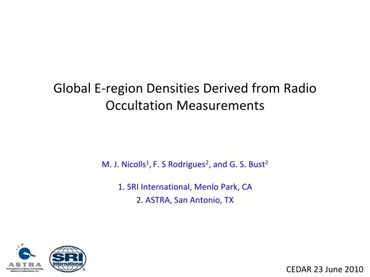
Global E-region Densities Derived from Radio Occultation Measurements. M. J. Nicolls 1 , F. S Rodrigues 2 , and G. S. Bust 2 1. SRI International, Menlo Park, CA 2. ASTRA, San Antonio, TX. CEDAR 23 June 2010. Overview. The main goals of this project are:

E N D
Global E-region Densities Derived from Radio Occultation Measurements • M. J. Nicolls1,F. S Rodrigues2, and G. S. Bust2 • 1. SRI International, Menlo Park, CA • 2. ASTRA, San Antonio, TX CEDAR 23 June 2010
Overview • The main goals of this project are: • Development and validation of an approach for estimation of E-region density profiles from radio occultation measurements that mitigates the effects of F-region density gradients. • Application of results for a better understanding of equatorial Spread F development and/or suppression.
Motivation • Lack of E-region measurements • Vertical sounders (~> 1 MHz, daytime) • ISRs (> ?) • Jicamarca – Paracasbistatic coherent radar (Daytime during EEJ only) • Good knowledge about the E-region density/conductivity around sunset times at low-latitude is crucial for modeling of low-latitude E-fields. • Good knowledge about the E-region conductivity is also important for estimation of the linear growth rate of equatorial spread F irregularities. • Many other aspects: • Better specification of the high-latitude E-region conductivities? • The latitudinal and longitudinal distribution of sporadic E layers is poorly known (e.g. Carrasco, 2005).
E-region and Equatorial Spread F The linear growth rate for the Generalized Rayleigh-Taylor instability can be given in terms of flux-tube integrated quantities [Zalezak and Ossakow, 1982]: Where E-region densities directly affect the conductivity term in the linear growth rate. COPEX Campaign in Brazil, 2005
From Fesen et al. 2000 Abdu (2001) E-region and Equatorial Spread F - The importance of the longitudinal (or local time) gradient in the E-region near sunset hours affects the occurrence of the so-called pre-reversal enhancement (PRE) of the zonal equatorial electric field. - The PRE plays (perhaps the most) important role in ESF development: Simulations suggest that PRE does not develop for ne(125km) > 7.5x10⁹m-3 but depends on longitudinal gradients + vertical profile
E-region and Equatorial Spread F • The occurrence of sporadic E layers at low latitudes can also affect (a) the conductivity term in GRT linear growth rate, and (b) the longitudinal gradient in conductivity. Therefore, they are also associated with ESF inhibition. • It is generally accepted that Es at mid-lats are produced by wind shear. • Much less is known about equatorial Es. • The formation of Es by long-lived metallic ions produced by meteor ionization has been suggested. • Studies of the correlation between meteor showers vs Es occurrence produced results varying between a negative to high a correlation (Malhotra et al. 2008)! • Es may also seed ESF via a Es-layer instability [Tsunoda, 2006]
The radio occultation technique Radio occultation measurements provide the TEC (ROTEC) along the raypath between a LEO satellite and a GPS satellite as a function of the height of the tangentpoint of the path. LEO 7 6 5 ht ht TEC profile 4 7 6 3 5 4 2 3 E-region 1 2 1 F-region GPS TEC
The radio occultation technique Now, if the distribution of electron density (ne) in the ionosphere were spherically symmetric, at least over the region we are interested, we could write: ne(lat, lon, h) = ne(r) And we can show that TEC(ht) would be given by the so-called Abel transform: Given TEC measurements, one can obtain ne(r) using theinverse Abel transform: ne(lat, lon, h) = ne(r) does not hold in most cases, and horizontal density gradients should be taken into account when trying to obtain estimates of ne(h)from RO TEC observations.
Estimating E-region profiles: An alternative approach LEO Assuming that spherical symmetry assumption only holds in the E-region we can write: s2 ht The measured TEC has contributions from the E and F regions: GPS s1 TECmeas = TECE-region + TECF-region or: Summary of Approach TECE-region = TECmeas - TECF-region E-region • IDA specification using available ground-based TEC and portion of occultations with tangent points >150 km • Estimation and removal of F-region contribution to rays that have E-region tangent points • Abel inversion of E-region portion of occultation • TECmeas are the RO measurements • TECF-region can be obtained from an assimilative model • ne(h) is obtained from Abel inversion of TECE-region F-region
Jicamarca Bistatic Experiment • Uses the Faraday rotation of an obliquely coherently scattered radar signal to determine within the equatorial electrojet (100-115 km) • Works during daytime, Relative Errors < 1% • Equatorial region is a good place for validation studies because general lack of sporadic ionization layers Hysell and Chau [2001]; Shume et al. [2005]
Example of Results Profile Comparison to Bistatic Radar JRO ✖ • Jicamarca-Paracas Bistatic Radar • Inversion • -.- FIRI • -- IRI Nicolls et al. (JGR, 2009)
Validation / Comparison Ne at 100, 105, and 110 km Red – Inversion, Blue – JRO-Paracas Location of occultations and rays that pass through the E-region Nicolls et al. (2009)
Error Analysis • Same volume radar-occultation observations were not possible. • Comparison of near observations suggest that errors are mostly around 2x10¹⁰ m-3 (fractional errors ~20%) • More importantly, errors decrease with distance from occultation to radar, suggesting that some of the errors are geophysical. Nicolls et al. (2009)
Estimating E-region profiles: An alternative approach • Possible issues with the proposed approach: • Accuracy of the F-region specification • Depends on the performance of the assimilative model • Depends on data availability • Lack of spherical symmetry in the E-region during sunset/sunrise? • One possible way to mitigate this effect is to select occultation with a small coverage (lat/lon) area. • Lack of spherical symmetry in the E-region caused by sporadic E-layers • Currently, there are few measurements in regards to the range of Sporadic-E layer spatial scales
Statistical/Climatological Results • Four full months were selected for a study of the global E-region and climatology analysis: Apr. 07, Jul. 07, Oct. 07, and Jan. 08. • Requires IDA runs and E-region inversions (1 IDA run takes about ¾ of a day; 1 month takes ~1-2 days). • Here we show results for April 2007 and January 2008. • Quality control: Only inversions with non-negative density values between 80 and 150 km altitude were considered. • Initially presented in Fall AGU poster, Rodrigues et al. [2009]
Statistical/Climatological Results Observations 1-25 April 2007 1-25 January 2008
Statistical/Climatological Results E-region (80-130 km) Vertical TEC – Apr 2007
Statistical/Climatological Results E-region (80-130 km) Vertical TEC – Jan 2008
Statistical/Climatological Results Ne vs Local Time – Apr 2007 (-20o < lat < 20o) Data – Mean – Median
Statistical/Climatological Results Ne vs Local Time – Jan 2008 (-20o < lat < 20o) Data – Mean – Median
Statistical/Climatological Results Ne vs Local Time – Apr 2007 (-20o < lat < 20o)
Statistical/Climatological Results Ne vs Local Time – Jan 2008 (-20o < lat < 20o)
Empirical Modeling Ne vs Solar zenith angle – Apr 2007 (-30o < lat < 30o) Mean Median
Empirical Modeling Ne vs Solar zenith angle – Jan 2008 (-30o < lat < 30o) Mean Median
Summary • Proposed an alternative methodology for inversion of E-region profiles. • We have successfully inverted daytime E-region density profiles. Comparison with radar measurements indicates accuracy better than 2x10¹⁰ m-3 using this new methodology. • Our new methodology has been used to obtain global and nighttime vertical density profiles at E-region heights. • Initial analysis shows the expected local time and seasonal variability of the E-region. • Nighttime densities under investigation; mean peak values of ~1-2x10¹⁰ m-3 Future Work: • - Finish climatological analysis + empirical modeling + variability specification • - Electric field modeling and variability specification using this climatology • - Case studies of Es inhibition of spread F + modeling of flux-tube integrated conductances to investigate effect on growth rates