Download
1 / 52
520 likes | 620 Views
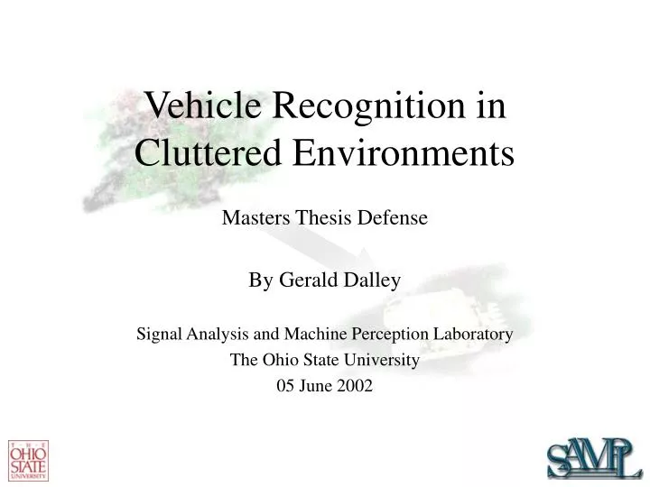
Vehicle Recognition in Cluttered Environments. Masters Thesis Defense By Gerald Dalley Signal Analysis and Machine Perception Laboratory The Ohio State University 05 June 2002. Overview. Problem Statement and Motivation Recognition Steps Range Image Generation

E N D
Vehicle Recognition in Cluttered Environments Masters Thesis Defense By Gerald Dalley Signal Analysis and Machine Perception Laboratory The Ohio State University 05 June 2002
Overview • Problem Statement and Motivation • Recognition Steps • Range Image Generation • Local Surface Estimation and Decimation • Global Surface Reconstruction • Surface Segmentation • Graph Matching • Conclusions and Future Work • Questions
“earthmover detected” Problem Statement and Motivation • Problem • Recognize vehicles • Military and civilian • Forested environment • Motivation • Hostile forces tend to hide • Camouflage and occlusion foil the human visual system
Range Image Generation:Overview • Objects modeled • Clutter models • Camera flight paths (scenes) • Noise generation Range Image Generation Local Surface Fitting Surface Reconstruction Surface Segmentation Graph Matching
earthmover obj1 sedan semi tank Range Image Generation: Objects Modeled
500 Discs • Radius of 100mm • Volume of 12.2 x 12.2 x 2 meters Range Image Generation: Clutter Models • Visually realistic trees • Look good, but… • Poor occlusion • Very long runtimes
Range Image Generation: Camera Flight Paths (Scenes) flyby circle unoccluded
Range Image Generation: Noise Generation • Isotropic additive Gaussian noise • Standard deviations of: • 0mm • 2mm • 4mm • 8mm • 16mm • 32mm
Local Surface Estimation and Decimation:Overview • Assumption: Vehicles are composed primarily of large, low-order, low-curvature surfaces. • Constraint: 10 tank views more than 220,000 range points (too many) • Point Selection (Decimation) • Principle Component Analysis • Biquadratic Surface Fits Range Image Generation Local Surface Estimation Surface Reconstruction Surface Segmentation Graph Matching
Local Surface Estimation and Decimation: Point Selection • Method 1: • Randomly select 1% (for example) of the original points • Make local surface estimates based on selected points • Problems: No noise σ = 0.3 Fit errors away from corner Fit errors due to noise Fit errors due to the corner Fit errors due to the corner
Local Surface Estimation and Decimation: Point Selection (cont’d.) Method 2: In the region of interest… • Collect range image points into cubic voxel bins (128x128x128mm) • Discard bins that have: • Too few points • Points that do not represent biquadratic surfaces well • Retain only the centroids of the bins and their surface fits
Local Surface Estimation and Decimation: Principle Component Analysis w u
Local Surface Estimation and Decimation: Biquadratic Surface Fits pi
Global Surface Reconstruction:Overview • Motivations • Post-Processing Range Image Generation Local Surface Fitting Surface Reconstruction Surface Segmentation Graph Matching
Global Surface Reconstruction:Motivations • Easy, unambiguous nearest-neighbor identification • Fast searches over small cardinality • Makes rendering easier • Avoids incorrect groupings of nearby surfaces
Surface Segmentation:Overview • Motivation: Correspondence is hard • Some Techniques Not Used • Spectral Clustering • An overview • Normalized cuts • Our affinity measure • Results Range Image Generation Local Surface Fitting Surface Reconstruction Surface Segmentation Graph Matching
Surface Segmentation:Some Techniques Not Used Robust Sequential Estimators (Mirza) Regions of Constant Curvature (Srikantiah)
Surface Segmentation:Overview of Spectral Clustering • Two surface points have an affinity… y1, where Ayi=li yi Aij
Graph Matching:Overview • Match tree example • Error measures • Entropy • Results • What caused problems? Range Image Generation Local Surface Fitting Surface Reconstruction Surface Segmentation Graph Matching
Graph Matching:Error Measures • Unary Error • Area, Elongation, Thickness • Orientation Error • How poorly pairs of normals match up • Centroid Distance Error • How poorly pairs of centroids match up • Cumulative Area Error • What percentage of the model area is not matched up
Graph Matching:What Caused Problems? • 19 total incorrect recognition results • 12: over-segmentation • 10: area errors (including non-existent segments)
Graph Matching:What Caused Problems? (cont’d.) • 4: mis-aligned segmentation
Conclusions • System features • Modular design • Handles pessimistic levels of clutter • 100% recognition on earthmover and sedan • Reliable segmentation is important when doing graph matching
Future Work • Articulation • Larger modelbase • Iterative recognition • Alternative segmentation methods • Other affinity matrix normalizations • Tensor voting • Enhanced version of Srikantiah’s algorithm • Verification • Alternative recognizers (e.g. SAI) • E3D! (hopefully, for the remaining SAMPL crowd)
Global Surface Reconstruction: Preliminaries:Voronoi Diagrams • Voronoi cell = locus of points closer to a given sample point than any other point
Global Surface Reconstruction: Preliminaries:Medial Axis • Medial axis = locus of points equidistant from at least two surface points (considering the original surface)
Global Surface Reconstruction: Preliminaries:ε-sampling • ε-sampling = Samples are at most ε times the distance to the medial axis
Global Surface Reconstruction:Cocone p+ • p+ ≡ pole of p = point in the Voronoi cell farthest from p • ε < 0.06 → • the vector from p to p+ is within π/8 of the true surface normal • The surface is nearly flat within the cell p Voronoi cell of p