Download

1 / 66
660 likes | 930 Views
The Medium Access Control Sublayer. Chapter 4. As we pointed out in Chap. 1, networks can be divided into two categories: those using point-to-point connections and those using broadcast channels. This chapter deals with broadcast networks and their protocols.

E N D
The Medium Access ControlSublayer Chapter 4
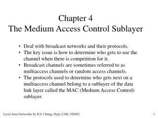
As we pointed out in Chap. 1, networks can be divided into two categories: those using point-to-point connections and those using broadcast channels. This chapter deals with broadcast networks and their protocols. In any broadcast network, the key issue is how to determine who gets to use the channel when there is competition for it. To make this point clearer, consider a conference call in which six people, on six different telephones, are all connected so that each one can hear and talk to all the others. It is very likely that when one of them stops speaking, two or more will start talking at once, leading to chaos. When only a single channel is available, determining who should go next is much harder. Many protocols for solving the problem are known and form the contents of this chapter. In the literature, broadcast channels are sometimes referred to as multiaccess channels or random access channels. The protocols used to determine who goes next on a multiaccess channel belong to a sublayer of the data link layer called the MAC (Medium Access Control) sublayer. The MAC sublayer is especially important in LANs, many of which use a multiaccess channel as the basis for communication. WANs, in contrast, use point-to-point links, except for satellite networks. Because multiaccess channels and LANs are so closely related, in this chapter we will discuss LANs in general, including a few issues that are not strictly part of the MAC sublayer. Technically, the MAC sublayer is the bottom part of the data link layer, so logically we should have studied it before examining all the point-to-point protocols in Chap. 3. Nevertheless, for most people, understanding protocols involving multiple parties is easier after two-party protocols are well understood. For that reason we have deviated slightly from a strict bottom-up order of presentation.
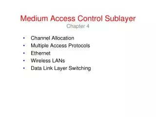
4.1 The Channel Allocation Problem • Static Channel Allocation in LANs and MANs • Dynamic Channel Allocation in LANs and MANs
4.1.1 Static Channel Allocation in LANs and MANs • FDM: The bandwidth is divided into N equal-sized portions . Each user is statically assigned one portion. • TDM: The time is divided into time slots. Each user is statically allocated every Nth time slot. • Static channel allocation methods do not work well with bursty traffic.
4.1.2 Dynamic Channel Allocation in LANs and MANs Before we get into the first of the many channel allocation methods to be discussed in this chapter, it is worthwhile carefully formulating the allocation problem. Underlying all the work done in this area are five key assumptions, described below. Station Model. The model consists of N independent stations (e.g., computers, telephones, or personal communicators), each with a program or user that generates frames for transmission. Stations are sometimes called terminals. The probability of a frame being generated in an interval of length Dt is lDt, where l is a constant (the arrival rate of new frames). Once a frame has been generated, the station is blocked and does nothing until the frame has been successfully transmitted. Single Channel Assumption. A single channel is available for all communication. All stations can transmit on it and all can receive from it. As far as the hardware is concerned, all stations are equivalent, although protocol software may assign priorities to them.
Collision Assumption. If two frames are transmitted simultaneously, they overlap in time and the resulting signal is garbled. This event is called a collision. All stations can detect collisions. A collided frame must be transmitted again later. There are no errors other than those generated by collisions. 4(a)Continuous Time. Frame transmission can begin at any instant. There is no master clock dividing time into discrete intervals. 4(b)Slotted Time. Time is divided into discrete intervals (slots). Frame transmissions always begin at the start of a slot. A slot may contain 0, 1, or more frames, corresponding to an idle slot, a successful transmission, or a collision, respectively. 5(a)Carrier Sense. Stations can tell if the channel is in use before trying to use it. If the channel is sensed as busy, no station will attempt to use it until it goes idle. 5(b)No Carrier Sense. Stations cannot sense the channel before trying to use it. They just go ahead and transmit. Only later can they determine whether the transmission was successful.
4.2 Multiple Access Protocols • ALOHA • Carrier Sense Multiple Access Protocols • Collision-Free Protocols • Limited-Contention Protocols • Wavelength Division Multiple Access Protocols • Wireless LAN Protocols
4.2.1 ALOHA In the 1970s, Norman Abramson and his colleagues at the University of Hawaii devised a new and elegant method to solve the channel allocation problem. Their work has been extended by many researchers since then (Abramson, 1985). Although Abramson's work, called the ALOHA system, used ground-based radio broadcasting, the basic idea is applicable to any system in which uncoordinated users are competing for the use of a single shared channel. We will discuss two versions of ALOHA here: • Pure ALOHA • Slotted ALOHA They differ with respect to whether time is divided into discrete slots into which all frames must fit. Pure ALOHA does not require global time synchronization; slotted ALOHA does.
Pure ALOHA The basic idea of an ALOHA system is simple: let users transmit whenever they have data to be sent. There will be collisions, of course, and the colliding frames will be damaged. However, due to the feedback property of broadcasting, a sender can always find out whether its frame was destroyed by listening to the channel, the same way other users do. With a LAN, the feedback is immediate; with a satellite, there is a delay of 270 msec before the sender knows if the transmission was successful. If listening while transmitting is not possible for some reason, acknowledgements are needed. If the frame was destroyed, the sender just waits a random amount of time and sends it again. The waiting time must be random or the same frames will collide over and over, in lockstep. Systems in which multiple users share a common channel in a way that can lead to conflicts are widely known as contention systems.
Pure ALOHA Stations cannot sense the channel before trying to use it. They just go ahead and transmit. Only later can they determine whether the transmission was successful. Fig.4-1 In pure ALOHA, frames are transmitted at completely arbitrary times.
Pure ALOHA Whenever two frames try to occupy the channel at the same time, there will be a collision and both will be garbled. If the first bit of a new frame overlaps with just the last bit of a frame almost finished, both frames will be totally destroyed and both will have to be retransmitted later. The checksum cannot (and should not) distinguish between a total loss and a near miss. Bad is bad. Fig.4-2 Vulnerable period for the shaded frame.
Slotted ALOHA In 1972, Roberts published a method for doubling the capacity of an ALOHA system (Roberts, 1972). His proposal was to divide time into discrete intervals, each interval corresponding to one frame. This approach requires the users to agree on slot boundaries. One way to achieve synchronization would be to have one special station emit a pip at the start of each interval, like a clock. In Roberts' method, which has come to be known as slotted ALOHA, in contrast to Abramson's pure ALOHA, a computer is not permitted to send whenever a carriage return is typed. Instead, it is required to wait for the beginning of the next slot. Thus, the continuous pure ALOHA is turned into a discrete one.
Performance of ALOHA System Fig.4-3 Throughput versus offered traffic for ALOHA systems.
4.2.2 Carrier Sense Multiple Access Protocols (CSMA) With slotted ALOHA the best channel utilization that can be achieved is 1/e. This is hardly surprising, since with stations transmitting at will, without paying attention to what the other stations are doing, there are bound to be many collisions. In local area networks, however, it is possible for stations to detect what other stations are doing, and adapt their behavior accordingly. These networks can achieve a much better utilization than 1/e. In this section we will discuss some protocols for improving performance. Protocols in which stations listen for a carrier (i.e., a transmission) and act accordingly are called carrier sense protocols. A number of them have been proposed. Kleinrock and Tobagi (1975) have analyzed several such protocols in detail. Below we will mention several versions of the carrier sense protocols.
Persistent and Nonpersistent CSMA The first carrier sense protocol that we will study here is called 1-persistent CSMA (Carrier Sense Multiple Access). When a station has data to send, it first listens to the channel to see if anyone else is transmitting at that moment. If the channel is busy, the station waits until it becomes idle. When the station detects an idle channel, it transmits a frame. If a collision occurs, the station waits a random amount of time and starts all over again. The protocol is called 1-persistent because the station transmits with a probability of 1 when it finds the channel idle. The propagation delay has an important effect on the performance of the protocol. There is a small chance that just after a station begins sending, another station will become ready to send and sense the channel. If the first station's signal has not yet reached the second one, the latter will sense an idle channel and will also begin sending, resulting in a collision. The longer the propagation delay, the more important this effect becomes, and the worse the performance of the protocol. Even if the propagation delay is zero, there will still be collisions. If two stations become ready in the middle of a third station's transmission, both will wait politely until the transmission ends and then both will begin transmitting exactly simultaneously, resulting in a collision. If they were not so impatient, there would be fewer collisions. Even so, this protocol is far better than pure ALOHA because both stations have the decency to desist from interfering with the third station's frame. Intuitively, this approach will lead to a higher performance than pure ALOHA. Exactly the same holds for slotted ALOHA.
A second carrier sense protocol is nonpersistent CSMA. In this protocol, a conscious attempt is made to be less greedy than in the previous one. Before sending, a station senses the channel. If no one else is sending, the station begins doing so itself. However, if the channel is already in use, the station does not continually sense it for the purpose of seizing it immediately upon detecting the end of the previous transmission. Instead, it waits a random period of time and then repeats the algorithm. Consequently, this algorithm leads to better channel utilization but longer delays than 1-persistent CSMA. The last protocol is p-persistent CSMA. It applies to slotted channels and works as follows. When a station becomes ready to send, it senses the channel. If it is idle, it transmits with a probability p. With a probability q = 1 - p, it defers until the next slot. If that slot is also idle, it either transmits or defers again, with probabilities p and q. This process is repeated until either the frame has been transmitted or another station has begun transmitting. In the latter case, the unlucky station acts as if there had been a collision (i.e., it waits a random time and starts again). If the station initially senses the channel busy, it waits until the next slot and applies the above algorithm. Figure 4-4 shows the computed throughput versus offered traffic for all three protocols, as well as for pure and slotted ALOHA.
Persistent and Nonpersistent CSMA Fig.4-4 Comparison of the channel utilization versus load for various random access protocols.
CSMA with Collision Detection Persistent and nonpersistent CSMA protocols are clearly an improvement over ALOHA because they ensure that no station begins to transmit when it senses the channel busy. Another improvement is for stations to abort their transmissions as soon as they detect a collision. In other words, if two stations sense the channel to be idle and begin transmitting simultaneously, they will both detect the collision almost immediately. Rather than finish transmitting their frames, which are irretrievably garbled anyway, they should abruptly stop transmitting as soon as the collision is detected. Quickly terminating damaged frames saves time and bandwidth. This protocol, known as CSMA/CD (CSMA with Collision Detection) is widely used on LANs in the MAC sublayer. Fig.4-5 CSMA/CD can be in one of three states: contention, transmission, or idle.
4.2.3 Collision-Free Protocols Collision-Free Protocols are protocols that resolve the contention for the channel without any collisions at all, not even during the contention period. In the protocols to be described, we assume that there are exactly N stations, each with a unique address from 0 to N - 1 ''wired'' into it. It does not matter that some stations may be inactive part of the time. We also assume that propagation delay is negligible. The basic question remains: Which station gets the channel after a successful transmission? We continue using the model of Fig. 4-5 with its discrete contention slots.
The Basic Bit-map Protocol In the basic bit-map protocol, station j may announce that it has a frame to send by inserting a 1 bit into slot j. After all N slots have passed by, each station has complete knowledge of which stations wish to transmit. At that point, they begin transmitting in numerical order. Since everyone agrees on who goes next, there will never be any collisions. Protocols like this in which the desire to transmit is broadcast before the actual transmission are called reservation protocols. Fig.4-6 The basic bit-map protocol.
Binary Countdown A problem with the basic bit-map protocol is that the overhead is 1 bit per station, so it does not scale well to networks with thousands of stations. We can do better than that by using binary station addresses. A station wanting to use the channel now broadcasts its address as a binary bit string, starting with the high-order bit. All addresses are assumed to be the same length. The bits in each address position from different stations are BOOLEAN ORed together. We will call this protocol binary countdown. To avoid conflicts, an arbitration rule must be applied: as soon as a station sees that a high-order bit position that is 0 in its address has been overwritten with a 1, it gives up.
An Example of Binary Countdown Fig. 4-7 The binary countdown protocol. A dash indicates silence.
4.2.4 Limited-Contention Protocols Under conditions of light load, contention (i.e., pure or slotted ALOHA) have low delay. As the load increases, contention’s channel efficiency gets worse . Just the reverse is true for the collision-free protocols. At low load, they have high delay, but as the load increases, the channel efficiency improves. Limited-contention protocolsuse contention at low load to provide low delay, but use a collision-free technique at high load to provide good channel efficiency. 1/e Fig.4-8 Acquisition probability for a symmetric contention channel.
4.3 Ethernet • Ethernet Cabling • Manchester Encoding • The Ethernet MAC Sublayer Protocol • The Binary Exponential Backoff Algorithm • Ethernet Performance • Switched Ethernet • Fast Ethernet • Gigabit Ethernet • IEEE 802.2: Logical Link Control • Retrospective on Ethernet
4.3.1 Ethernet Cabling Since the name ''Ethernet'' refers to the cable (the ether), let us start our discussion there. Four types of cabling are commonly used, as shown in Fig. 4-13. Fig.4-13 The most common kinds of Ethernet cabling.
Three Kinds of Ethernet Cabling Fig.4-14 (a) 10Base5, (b) 10Base2, (c) 10Base-T.
Cable Topologies In Fig. 4-15(a), a single cable is snaked from room to room, with each station tapping into it at the nearest point. In Fig. 4-15(b), a vertical spine runs from the basement to the roof, with horizontal cables on each floor connected to the spine by special amplifiers (repeaters). In some buildings, the horizontal cables are thin and the backbone is thick. The most general topology is the tree, as in Fig. 4-15(c). Each version of Ethernet has a maximum cable length per segment. To allow larger networks, multiple cables can be connected by repeaters, as shown in Fig. 4-15(d). Fig.4-15 (a) Linear, (b) Spine, (c) Tree, (d) Segmented.
4.3.2 Manchester Encoding None of the versions of Ethernet uses straight binary encoding with 0 volts for a 0 bit and 5 volts for a 1 bit because it leads to ambiguities. Two widely used approaches are called Manchester encoding and differential Manchester encoding. With Manchester encoding, each bit period is divided into two equal intervals. A binary 1 bit is sent by having the voltage set high during the first interval and low in the second one. A binary 0 is just the reverse: first low and then high. This scheme ensures that every bit period has a transition in the middle, making it easy for the receiver to synchronize with the sender. A disadvantage of Manchester encoding is that it requires twice as much bandwidth as straight binary encoding because the pulses are half the width. For example, to send data at 10 Mbps, the signal has to change 20 million times/sec. In differential Manchester encoding , a 1 bit is indicated by the absence of a transition at the start of the interval. A 0 bit is indicated by the presence of a transition at the start of the interval. In both cases, there is a transition in the middle as well. The differential scheme requires more complex equipment but offers better noise immunity. All Ethernet systems use Manchester encoding due to its simplicity.
4.3.2 Manchester Encoding Fig.4-16 (a) Binary encoding, (b) Manchester encoding, (c) Differential Manchester encoding.
4.3.3 Ethernet MAC Sublayer Protocol The original DIX (DEC, Intel, Xerox) frame structure is shown in Fig. 4-17(a). Each frame starts with a Preamble of 8 bytes, each containing the bit pattern 10101010. The Manchester encoding of this pattern produces a 10-MHz square wave for 6.4 µsec to allow the receiver's clock to synchronize with the sender's. They are required to stay synchronized for the rest of the frame, using the Manchester encoding to keep track of the bit boundaries. The IEEE 802.3 frame structure has two changes to the DIX format, as shown in Fig. 4-17(b). The first one was to reduce the preamble to 7 bytes and use the last byte for a Start of Frame delimiter, for compatibility with 802.4 and 802.5. The second one was to change the Type field into a Length field. Fig.4-17 Frame formats. (a) DIX Ethernet, (b) IEEE 802.3.
Ethernet Adresses The frame contains two addresses, one for the destination and one for the source. The standard allows 2-byte and 6-byte addresses, but the parameters defined for the 10-Mbps baseband standard use only the 6-byte addresses. The high-order bit of the destination address is a 0 for ordinary addresses and 1 for group addresses. Group addresses allow multiple stations to listen to a single address. When a frame is sent to a group address, all the stations in the group receive it. Sending to a group of stations is called multicast. The address consisting of all 1 bits is reserved for broadcast. A frame containing all 1s in the destination field is accepted by all stations on the network. The difference between multicast and broadcast is important enough to warrant repeating. A multicast frame is sent to a selected group of stations on the Ethernet; a broadcast frame is sent to all stations on the Ethernet. Multicast is more selective, but involves group management. Broadcasting is coarser but does not require any group management. Another interesting feature of the addressing is the use of bit 46 (adjacent to the high-order bit) to distinguish local from global addresses. Local addresses are assigned by each network administrator and have no significance outside the local network. Global addresses, in contrast, are assigned centrally by IEEE to ensure that no two stations anywhere in the world have the same global address. With 48 - 2 = 46 bits available, there are about 7 x 10¹³ global addresses. The idea is that any station can uniquely address any other station by just giving the right 48-bit number.
Type and Length field Next comes the Type field, which tells the receiver what to do with the frame. Multiple network-layer protocols may be in use at the same time on the same machine, so when an Ethernet frame arrives, the kernel has to know which one to hand the frame to. The Type field specifies which process to give the frame to. In IEEE 802.3, comes the Length field, which tells the length of Data. In 1997 IEEE said that both ways were fine with it. Fortunately, all the Type fields in use before 1997 were greater than 1500. Consequently, any number there less than or equal to 1500 can be interpreted as Length, and any number greater than 1500 can be interpreted as Type.
Data and Checksum Field Next come the data, up to 1500 bytes. In addition to there being a maximum frame length, there is also a minimum frame length, 46 bytes. If the data portion of a frame is less than 46 bytes, the Pad field is used to fill out the frame to the minimum size. . The final Ethernet field is the Checksum. It is effectively a 32-bit hash code of the data. If some data bits are erroneously received (due to noise on the cable), the checksum will almost certainly be wrong and the error will be detected. The checksum algorithm is a cyclic redundancy check (CRC) of the kind discussed in Chap. 3. It just does error detection, not forward error correction.
The Minimum Length of The Ethernet Frame When a transceiver detects a collision, it truncates the current frame, which means that stray bits and pieces of frames appear on the cable all the time. To make it easier to distinguish valid frames from garbage, Ethernet requires that valid frames must be at least 64 bytes long, from destination address to checksum, including both. Another (and more important) reason for having a minimum length frame is to prevent a station from completing the transmission of a short frame before the first bit has even reached the far end of the cable, where it may collide with another frame. This problem is illustrated in Fig. 4-18. Figure 4-18. Collision detection can take as long as 2t.
4.3.4 The Binary Exponential Backoff Algorithm when a collision occurs,the sender waits random time :t= 0~2i-1(2t ) i : number of collisions 2t: worst-case round-trip propagation time After ten collisions have been reached, the randomization interval is frozen at a maximum of 1023 slots. After 16 collisions, the controller throws in the towel and reports failure back to the computer. Further recovery is up to higher layers.
4.3.5 Ethernet Performance Fig.4-19 Efficiency of Ethernet at 10 Mbps with 512-bit slot times.
4.3.6 Switched Ethernet As more and more stations are added to an Ethernet, the traffic will go up. Eventually, the LAN will saturate. One way out is to go to a higher speed, say, from 10 Mbps to 100 Mbps. But with the growth of multimedia, even a 100-Mbps or 1-Gbps Ethernet can become saturated. Fortunately, there is an additional way to deal with increased load: switched Ethernet, as shown in Fig. 4-20. The heart of this system is a switch containing a high-speed backplane and room for typically 4 to 32 plug-in line cards, each containing one to eight connectors. Most often, each connector has a 10Base-T twisted pair connection to a single host computer. Fig.4-20 A simple example of switched Ethernet.
When a station wants to transmit an Ethernet frame, it outputs a standard frame to the switch. The plug-in card getting the frame may check to see if it is destined for one of the other stations connected to the same card. If so, the frame is copied there. If not, the frame is sent over the high-speed backplane to the destination station's card. The backplane typically runs at many Gbps, using a proprietary protocol. What happens if two machines attached to the same plug-in card transmit frames at the same time? It depends on how the card has been constructed. One possibility is for all the ports on the card to be wired together to form a local on-card LAN. Collisions on this on-card LAN will be detected and handled the same as any other collisions on a CSMA/CD network—with retransmissions using the binary exponential backoff algorithm. With this kind of plug-in card, only one transmission per card is possible at any instant, but all the cards can be transmitting in parallel. With this design, each card forms its own collision domain, independent of the others. With only one station per collision domain, collisions are impossible and performance is improved. With the other kind of plug-in card, each input port is buffered, so incoming frames are stored in the card's on-board RAM as they arrive. This design allows all input ports to receive (and transmit) frames at the same time, for parallel, full-duplex operation, something not possible with CSMA/CD on a single channel. Once a frame has been completely received, the card can then check to see if the frame is destined for another port on the same card or for a distant port. In the former case, it can be transmitted directly to the destination. In the latter case, it must be transmitted over the backplane to the proper card. With this design, each port is a separate collision domain, so collisions do not occur. Since the switch just expects standard Ethernet frames on each input port, it is possible to use some of the ports as concentrators. In Fig. 4-20, the port in the upper-right corner is connected not to a single station, but to a 12-port hub.
4.3.7 Fast Ethernet The basic idea behind fast Ethernet was simple: keep all the old frame formats, interfaces, and procedural rules, but just reduce the bit time from 100 nsec to 10 nsec, thus 100Mbps can be acquired. Fig.4-21 The original fast Ethernet cabling.
4.3.8 Gigabit Ethernet Gigabit Ethernet was ratified by IEEE in 1998 under the name 802.3z. The 802.3z committee's goals were essentially the same as the 802.3u committee's goals: make Ethernet go 10 times faster yet remain backward compatible with all existing Ethernet standards. Fig.4-22 (a) A two-station Ethernet. (b) A multistation Ethernet.
Gigabit Ethernet Gigabit Ethernet supports both copper and fiber cabling, as listed in Fig. 4-23. Signaling at or near 1 Gbps over fiber means that the light source has to be turned on and off in under 1 nsec. LEDs simply cannot operate this fast, so lasers are required. Two wavelengths are permitted: 0.85 microns (Short) and 1.3 microns (Long). Lasers at 0.85 microns are cheaper but do not work on single-mode fiber. Fig.4-23 Gigabit Ethernet cabling.
4.3.9 IEEE 802.2: Logical Link Control In Chap. 3, we saw how two machines could communicate reliably over an unreliable line by using various data link protocols. These protocols provided error control (using acknowledgements) and flow control (using a sliding window). In contrast, in this chapter, we have not said a word about reliable communication. All that Ethernet and the other 802 protocols offer is a best-efforts datagram service. Sometimes, this service is adequate. Nevertheless, there are also systems in which an error-controlled, flow-controlled data link protocol is desired. IEEE has defined one that can run on top of Ethernet and the other 802 protocols. In addition, this protocol, called LLC (Logical Link Control), hides the differences between the various kinds of 802 networks by providing a single format and interface to the network layer. This format, interface, and protocol are all closely based on the HDLC protocol we studied in Chap. 3. LLC forms the upper half of the data link layer, with the MAC sublayer below it, as shown in Fig. 4-24.
4.3.9 IEEE 802.2: Logical Link Control Fig.4-24 (a) Position of LLC. (b) Protocol formats.
4.4 Wireless LANs :802.11 4.5 Broadband Wireless: 802.16 4.6 Bluetooth:802.15Other 802 Protocols:802.4,802.5,802.6
4.7 Data Link Layer Switching Many organizations have multiple LANs and wish to connect them. LANs can be connected by devices called bridges, which operate in the data link layer. Bridges examine the data layer link addresses to do routing. Since they are not supposed to examine the payload field of the frames they route, they can transport IPv4 (used in the Internet now), IPv6 (will be used in the Internet in the future), AppleTalk, ATM, OSI, or any other kinds of packets. In contrast, routers examine the addresses in packets and route based on them. Although this seems like a clear division between bridges and routers, some modern developments, such as the advent of switched Ethernet, have muddied the waters, as we will see later. In the following sections we will look at bridges and switches, especially for connecting different 802 LANs. There are six reasons why a single organization may end up with multiple LANs.
Fig.4-39 Multiple LANs connected by a backbone to handle a total load higher than the capacity of a single LAN.
4.7.1 Bridges from 802.x to 802.y How does a bridge work ? Fig.4-40 Operation of a LAN bridge from 802.11 to 802.3.
So far it looks like moving a frame from one LAN to another is easy. Such is not the case. Each of the LANs uses a different frame format (see Fig. 4-41). As a result, any copying between different LANs requires reformatting, which takes CPU time, requires a new checksum calculation, and introduces the possibility of undetected errors due to bad bits in the bridge's memory. Fig.4-41 The IEEE 802 frame formats. The drawing is not to scale.
4.7.2 Local Internetworking Fig.4-42 A configuration with four LANs and two bridges.
Routing Procedure When a frame arrives, a bridge must decide whether to discard or forward it, and if the latter, on which LAN to put the frame. This decision is made by looking up the destination address in a big (hash) table inside the bridge. The table can list each possible destination and tell which output line (LAN) it belongs on. For example, B2's table would list A as belonging to LAN 2, since all B2 has to know is which LAN to put frames for A on. That, in fact, more forwarding happens later is not of interest to it. The routing procedure for an incoming frame depends on the LAN it arrives on (the source LAN) and the LAN its destination is on (the destination LAN), as follows: • If destination and source LANs are the same, discard the frame. • If the destination and source LANs are different, forward the frame. • If the destination LAN is unknown, use flooding.