Download
1 / 110
1.19k likes | 1.5k Views
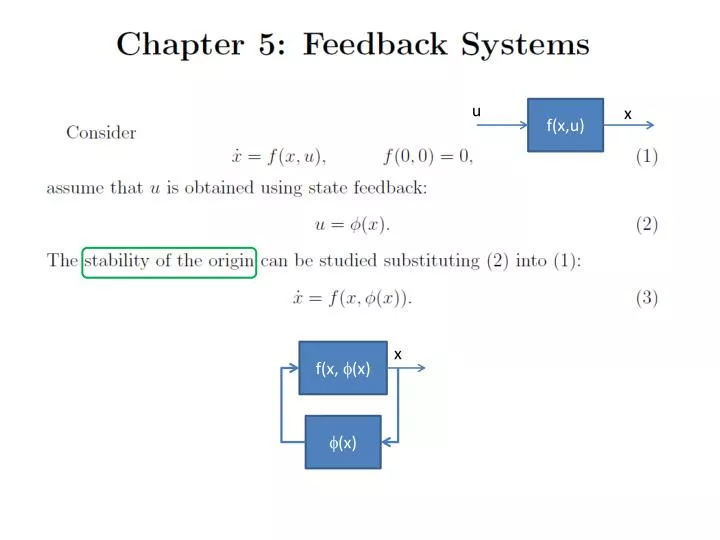
u. f( x,u ). x. x. f(x, (x ). (x). Example: Using feed-forward, what should be canceled?. Example: Using feed-forward, what should be canceled?. Example System: Electric Motor. Each link is basically a brushed DC motor with a pendulum load. Motivating Example: Brushed DC Motor.

E N D
u f(x,u) x x f(x, (x) (x)
Example System: Electric Motor Each link is basically a brushed DC motor with a pendulum load
Motivating Example: Brushed DC Motor Overview Apply voltage Produces current Produces Torque Rotates Mechanical Link q(t) is the angular load position i(t) is the coil current Torque Mechanical Subsystem (Pendulum-like arm) Electrical Subsystem (Motor Winding)
Motivating Example: Brushed DC Motor Mechanical subsystem Electrical subsystem Connection between subsystems
Motivating Example: Brushed DC Motor Traditional velocity control design using feedback linearization considering only the mechanical dynamics with an inertial load, like a wheel or fan (not a pendulum, N=0 in general model) Design control using Lyapunov analysis tools to drive speed to zero Propose a quadratic Lyapunov function (could use any function that works with our Theorems) M just to simplify the algebra (but it does affect the control) Note that the motor would actually slow to zero even if there is no torque (control) input
Motivating Example: Brushed DC Motor Design control to drive same system to a non-zero speed P (P is the desired speed) using a change of variables
Motivating Example: Brushed DC Motor Position control of the motor with robotic load but ignoring the electrical dynamics State space form Torque indirectly affects the position x1 Problem: need -x12 here Address this using Integrator Backstepping
Motivating Example: Brushed DC Motor Address this using Integrator Backstepping
Motivating Example: Brushed DC Motor Most electric motors fit into this same framework such as brushless DC, wound field DC, AC, stepper motor, induction motor Complication is that the other motor types have multiple windings (phases) An electronic or mechanical commutation is required to switch between phases to produce torque
Consider this first
5 i.e. add zero to (7) System after adding and subtracting
Change of variables: You can think of this new variable as the error between the j(x) that you would like to apply and the x that actually is applied, i.e. a tracking error
Recall: No control input in (15) v v Now design vto stabilize the system (with statesz, x)
(7) (8) We have embedded the problem that we said we could solve (first-order system) The transformed system (with statesz,x) is now stabilized; however, v is not the input to our real system (can’t apply v to our system)
Derivative of the control for the first subsystem This is now a formula for solving the problem of the specific form given in (7) and (8)
We already solved a similar problem in Example 1: We are embedding the control design approach, “Basic Feedback Linearization”, into the Integrator Backstepping. Other control design techniques could be used here.
Formula for u Formula for V PD? Yes Radially Unbounded? yes
Alternate Solution to Example 4 (Handcrafted Backstepping) Motivated by tracking error: - Desired trajectory that we can specify to control x1 Error between actual trajectory x2 and the desired trajectory (See Example 4) To this point:We have stabilized x1if we know that the tracking error η2 goes to zero. Must now work with the input u to make certain that η2 goes to zero.
Alternate Solution to Example 4 (Handcrafted Backstepping) = 1 1 - + - + Note: This is a dynamic system that describes the tracking error - we want to prove that the state of this system will to go to zero (is stable at zero) just like the systems we analyzed in Chapters 3. Stabilizing term Additional requirements in the composite Lyapunov analysis
Alternate Solution to Example 4 (Handcrafted Backstepping) Could not remove this interconnection term earlier because it allowed us to introduce x2d into the x1 dynamics. 1 (same result as Example 4 with k=1)
We have solved the backstepping problem for a specific class of systems: No other terms but u Scalar Showed a general approach that provides formulas for u and V Showed a handcrafted approach.
Solution of the more complicated problem in this form can be solved as a recursion of the simple solution (one coupled subsystem) Must now apply the control through 2 subsystems
Alternate Solution to Example 6 (Handcrafted Backstepping) -cont
Alternate Solution to Example 6 (Handcrafted Backstepping) -cont
Alternate Solution to Example 6 (Handcrafted Backstepping) -cont
Alternate Solution to Example 6 (Handcrafted Backstepping) -cont Control design Operation of Control
Alternate Solution to Example 6 (Handcrafted Backstepping) - Simulation x1 x3 x2
Alternate Solution to Example 6 (Handcrafted Backstepping) - Simulation Eta 3 Eta 2
If g(x)=0 the system is not controllable Electric Motor Mechanical Dynamics Electrical Dynamics