Download
1 / 44
440 likes | 586 Views
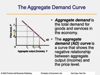
ECON 3410/4410 LECTURE 7 Aggregate demand dynamics. Ragnar Nymoen 4 October 2007. Overview. Review of aggregate demand and its components. Closed economy, open economy in a later lecture

E N D
ECON 3410/4410 LECTURE 7Aggregate demand dynamics Ragnar Nymoen 4 October 2007
Overview • Review of aggregate demand and its components. • Closed economy, open economy in a later lecture • Determinants of aggregate investments (ch 15) and consumption (ch 16), important and volatile components of aggregate demand • Aggregate demand put together, • and how monetary policy affects aggregate demand (ch 17)---the transmission mechanism. • Term structure of interest rates • Regime dependency of AD curve • Aggregate demand and aggregate supply • Short and long-run versions of the closed economy AS-AD model
Overview of Q-theory of investment • The market value of a firm is determined by discounting future dividends to the owners • By investing in capital, the firm grows and hence its capacity to generate dividends increases • The cost of investing one unit of capital is exogenous • This provides an incentive for firms with a high market value per unit of capital to invest • Definition: q = the ratio between the market value of the firm (V) and the replacement value of its capital stock (K) • Note: Q-theory applied to housing investment (section 15.4) is cursory (you may drop it)
Pricing by arbitrage condition • Arbitrage condition: In every period, stocks and bonds must yield the same risk-adjusted rate of return Vt = real stock market value of the firm at the start of period t Vet+1 = expected real stock market value of the firm at the start of period t+1 De = real expected dividend at the end of the period t r = real interest rate on bonds = risk premium on shares • In this way, markets for financial captial and real captial becomes integrated.
The fundamental value of a firm • Successive substitution of Vet+j gives: • Assume that the future value of the firm Vet+1 cannot rise faster than r + (else it would be of infinite value), i.e.:
The fundamental value of a firm • Then the infinite sum can be written as: • What does this expression remind you of? • Interpretation: The fundamental value of the firm equals the present value of expected future dividends • The role of the interest rate: We only assume that the expected return on shares is systematically related to the return on bonds • What about investments? The firm must decide whether to pay out its profits now (as dividends) or invest it in order to increase profits(dividends) later: Maximize Vt with respect to It
The decision to invest • Definition: qt = Vt / Kt = the ratio between the market value of the firm and the replacement value of its capital stock • Expected value of the firm tomorrow: where we have used: and • Cash flow constraint: e = expected profit c = installation costs • Assume the following installation cost function:
Optimal level of investment depends on q • Maximization of Vt taking qt as given gives the following first-order conditions:
An example of the investment function • Assume that in order to simplify the value of the firm to • Assume furthermore that and = expected dividend pay-out ratio = constant profit share • Using the definition of q this gives the investment function
The general investment function • Abstracting from the functional form the general investment function is: E = index of business confidence • Note that the risk premium is omitted • Note that in ch. 17 the level of capital K is assumed constant and the notation changes slightly ( is the index of business confidence)
Static investment function • Note that the rationale for assuming K constant (despite Kt=Kt-1 +It) is that K is a stock variable, while I is a flow variable. • Hence Kt is close to Kt-1 if the time period is short, even for large It • However, as we shall see, Itmay still react ”dynamically” because of dynamics elsewhere in the full model.
Overview of intertemporal consumption theory • Diminishing marginal utility of consumption provides an incentive for consumption smoothing over time. • Through the capital market, consumers can save or borrow and thus separate consumption from current income. • The discounted value of disposable lifetime income (human wealth) plus the initial stock of financial wealth represents the consumer’s lifetime budget constraint. • In optimum the consumer is indifferent between consuming an extra unit today and saving that extra unit in order to consume it tomorrow. • Current consumption will be proportional with wealth – not income. • Note: Issues on debt-financed tax cuts and Ricardian equivalence will be treated later on in the course.
Intertemporal consumer preferences • Representative consumer with a two-period utility function • Properties of the utility function: • the marginal utility of consumption in each period is positive, but diminishing (provides an incentive for consumption smoothing) • the consumer is impatient: the rate of time preference is positive
Intertemporal budget constraint • Period 1 budget constraint • Period 2 budget constraint • The consumer’s intertemporal budget constraint V = financial wealth r = real rate of interest YL = labour income T = net tax payment (taxes minus transfers) C = consumption
Human wealth and financial wealth • V1 represents the consumer’s initial financial wealth • The present value of disposable lifetime income can be thought of as human wealth (or human capital) H • This simplifies the notation of the intertemporal budget constraint
Optimal intertemporal consumption • Utility over the consumer’s life-time becomes (as a function of C1) • Maximization of U with respect to C1 gives the following first-order conditions: • The Keynes-Ramsey rule:
Optimal intertemporal consumption • In optimum, the marginal rate of substitution between present and future consumption (MRS) must equal the relative price of present consumption (1+r)
Example of the consumption function with CES utility • The constant (intertemporal) elasticity of substitution utility function • u’(Ct) = Ct-1/ • Insert this into the Keynes-Ramsey rule
Example of the consumption function with CES utility • Insert the expression for the optimal C2 in terms of C1 into the intertemporal budget constraint. • Current consumption C1 is proportional to total current wealth (not current income). • The propensity to consume wealth is positive, but less than one.
The general consumption function g = growth rate of income (increases human wealth) • Some consumers may be credit constrained, hence Y1d • In chpt. 17 notation is slightly changed: • The value of financial wealth is treated implicitly in r • is an index of consumer confidence (proxy for expected income growth)
Relationship to consumtion function in IDM • In IDM we had a consumption function with fewer explanatory variables, essentially only arguments, only Y-T. • We could have added r, for example, but left it out for simplicity. • On the other hand we introduced lagged C of course • The IDM specification thus assumes that adjustment of C to changes in Y-T for example is all done within the period of analysis.
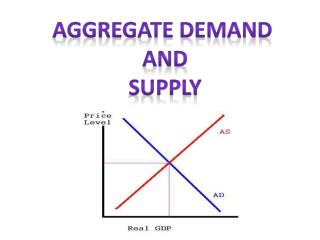
Overview over aggregate demand theory with endogenous monetary policy • Private investments and consumption are sensitive to changes in the real interest rate, hence there is a potential for stabilization policy • The government cares about stabilizing both output and inflation • In order to achieve the government’s objectives, the central bank sets the nominal short-term interest rate according to a Taylor rule • The resulting aggregate demand curve will be downwards-sloping in (y;) space • Important properties of the aggregate demand curve (the exact slope as well as the shift properties) will depend on the policy priorities (implied by the choice of coefficients in the Taylor rule) • Note: We will return to questions about fiscal policy (public consumption and taxes) later in the course
Equilibrium condition in the goods market gives the aggregate demand function Y • Investments plus consumption = aggregate private demand D • Equlibrium condition for the goods market (closed economy) • Properties of the aggregate private demand function
Evidence from Denmark seem to confirm a close relationship between private sector demand and the real interest rate over time The real interest rate and the private sector savings surplus in Denmark, 1971-2000. Per cent Source: Erik Haller Pedersen, ‘Udvikling i og måling af realrenten’, Danmarks Nationalbank, Kvartalsoversigt, 3. kvartal, 2001, Figure 6
The long-run aggregate demand function in log-linearized form • Assume that for that all arguments in the demand function are at their long-run (steady state) values, then long-run aggregate demand function is: • The IAM textbook shows how the aggregate demand function Y can be log-linearized around its long-run equilibrium values to give
The real and the nominal interest rate • The definition of the expected real interest rate • As long as i and are close to zero, we can approximate the real interest rate • As a first approach we will assume static expectations
The Taylor-rule as a proxy for monetary policy • History shows that governments care about stabilizing both output and inflation. • As a proxy for these policy motives, we can use the following interest rate rule proposed by John Taylor • With this rule, y, and r will be on their long-run equilibrium values on average. • * is interpreted as the inflation target (can be implicit or explicit). • For the stability of this economy, the parameter must be h positive so that an increase in inflation triggers an increase in the real interest rate (the Taylor principle).
Evidence from the euro area seems to confirm the Taylor rule as a proxy for monetary policy The 3 month nominal interest rate and an estimated Taylor rate for the euro area, 1999-2003. Per cent Source: Centre for European Policy Studies, Adjusting to Leaner Times, 5th Annual Report of the CEPS Macroeconomic Policy Group, Brussels, July 2003
Policy priorities implied by the Taylor rule coefficients seem to vary across countries Estimated interest rate reaction functions of four central banks 1. Source: Richard Clarida, Jordi Gali and Mark Gertler, ‘Monetary Policy Rules in Practice – Some International Evidence’, European Economic Review, 42, 1998, pp. 1033–1067. 2. Source: Centre for European Policy Studies, Adjusting to Leaner Times, 5th Annual Report of the CEPS Macroeconomic Policy Group, Brussels, July 2003.
and where Aggregate demand curve with endogenous monetary policy • The log-linearized version of the aggregate demand function Y and the Taylor rule can be combined to an aggregate demand curve in (y;) space
The shape of the aggregate demand curve will depend on the priorities of monetary policy Illustration of the aggregate demand curve under alternative monetary policy regimes (indicated by the choice of coefficients h and b in the Taylor rule)
The transmission mechanism: Term structure of interest rates • Remember that the rate of interest r in the demand function is interpretaable as an yield on long term bonds (10 years for example), a so called long interest rates • What monetary policy controls (directly or indirectly) is the very short interest rate, the money-market interest rate. • How can the central bank control the interest rate which is relevant for aggregate demand? • Answer: No worry! When capital markets are operating according to theory a change in the money market rate will be transmitted automatically to the long rates! • Arbitrage is (again) the mechanism
The expectations theory of the term structure of interest rates • Investment decisions depend on the expected cost of capital over the entire life of the asset (easily +10 years) • To what extend does the short-term policy rate influence long-term interest rates? • If short-term and long-term bonds are perfect substitutes (risk neutral investors) then the following arbitrage condition will hold • Taking logs and using the approximation ln(1+i) I • Alternative: Static interest rate expectations
In 2001, U.S. long-term interest rates kept a steady level as the short-term policy rate fell The Federal funds target rate (U.S. policy rate) and the yield on 10 year U.S. government bonds, 2001-2002. Per cent Source: Danmarks Nationalbank
Whatever happened to the money market? • The Taylor-rule pushes the money market that we know from the IS-LM model “into the background”. • This is OK in many ways, as long as it does not lead to misunderstanding like • “There is no role for money in the model” • The money market is always, there it is only that it is not always specified explixtely.
The money market in a period-to-period equilibirum Real Money supply i Real money demand L(Yt,it) Mt/Pt
Consider a money targeting regime: In each period the money supply is set by the central bank. Real Money supply in period t i Interest rate in peride t Real money demand L(Yt,it) Mt/Pt
Interest rate function in a money targeting regime The money graph in previous slide defines: it = i(Yt, Mt/Pt) where Y and M/P are regarded as determined outside the money market, M/P being the policy instrument. • If we define a long-run interest rate by inserting the long run values of the arguments in the i-function and then take the deviation between it and the long-run rate, we obtain a function that is qualitatively similar to the Taylor-rule. With one important difference: • In the money targeting regime the derivatives of the i-function are already given by the properties of the money demand function. • In the Taylor-rule the corresponding parameters h and b transpiresto be “free parameters”, to the chosen by the central bank (see next lecture) • Note: IAM p 504-506 contains a more detailed comparison/derivation of the two interest rate functions
The money market with a policy determined interest rate If the coefficients of the Taylor-rule are “free-parameters”, the money market operates like this: i Interest rate in period t M/P Real money supply In period t Real money supply is then an endogenous variable. Since the price level is pre-determined in any given period, it is the nominal money stock that adjusts immediately to bring the market into equilibrium. The Central Bank does this by market operations.
The AD-schedule is regime dependent • Although it is OK for some purposes to use the Taylor-rule as a “catch all” for monetary policy, as IAM does, it is also obscuring the important fact that • The response of aggregate demand (the impact multipliers of you like) to for example an increase in g is dependent on the monetary policy regime. • This point is going to be even more important when we later move to the open economy.
Aggregate demand dynamics---where is it? • This lecture was titled aggregate demand dynamics • But the main impression is that we have simplified so much that dynamics have almost been removed from the demand side. • Still there is one source of dynamics left: the real interest rate is and expectations variable---which is a source of dynamics. • In the next lecture we will utilize this to establish a long-run and a short-run version of the AD-AS model. • We will also consider a different model altogether: the real-business cycle model, where dynamics stems form other sources than expectations.