Download

1 / 52
520 likes | 623 Views
Pre-processing - Normalization Databases . Statistics for Microarray Data Analysis – Lecture 2 The Fields Institute for Research in Mathematical Sciences May 25, 2002. Biological question. Experimental design. Microarray experiment. Image analysis. Normalization. Analysis. Clustering.

E N D
Pre-processing - NormalizationDatabases Statistics for Microarray Data Analysis – Lecture 2 The Fields Institute for Research in Mathematical Sciences May 25, 2002
Biological question Experimental design Microarray experiment Image analysis Normalization Analysis Clustering Discrimination Estimation Testing Biological verification and interpretation
Begin by looking at the data • Was the experiment a success? • What analysis tools should be used? • Are there any specific problems?
Red/Green overlay images Co-registration and overlay offers a quick visualization, revealing information on colour balance, uniformity of hybridization, spot uniformity, background, and artifiacts such as dust or scratches Good: low bg, lots of d.e. Bad: high bg, ghost spots, little d.e.
Always log, always rotate log2R vs log2G M=log2R/G vs A=log2√RG
Histograms Signal/Noise = log2(spot intensity/background intensity)
Serious time of printing effects spot number Another data set, green channel intensities (log2G). Printed over 4.5 days.
Normalization • Why? • To correct for systematic differences between samples on the same slide, or between slides, which do not represent true biological variation between samples. • How do we know it is necessary? • By examining self-self hybridizations, where no true differential expression is occurring. • We find dye biases which vary with overall spot intensity, location on the array, plate origin, pins, scanning parameters,….
Self-self hybridizations False color overlay Boxplots within pin-groups Scatter (MA-)plots
A series of non self-self hybridizations From the NCI60 data set Early Ngai lab, UC Berkeley Early Goodman lab, UC Berkeley Early PMCRI, Melbourne Australia
Normalization • Within-slides • Which genes to use? • Location normalization • Scale normalization • Paired-slides (dye-swap) • Self-normalization • Between-slides
Which spots to use? • All genes on the array. • Constantly expressed genes (housekeeping). • Controls • Spiked controls (e.g. plant genes); • Genomic DNA titration series. • Rank invariant set.
Which spots to use, cont.? The LOWESS lines can be run through many different sets of points, and each strategy has its own implicit set of assumptions justifying its applicability. For example, we can justify the use of a global LOWESS approach by supposing that, when stratified by mRNA abundance, a) only a minority of genes are expected to be differentially expressed, or b) any differential expression is as likely to be up-regulation as down-regulation. Print-tips-group LOWESS requires stronger assumptions: that one of the above applies within each print-tip-group. The use of other sets of genes, e.g. control or housekeeping genes, involve similar assumptions.
Location normalization log2R/G log2R/G - c = log2R/ (kG) Standard practice (in most software) c is a constant such as the mean or median log ratio. Our preference c is a function of overall spot intensity A and print-tip group, and possibly other variables. Compute c by robust locally weighted regression of M On these variables. E.g. lowess.
Location normalization: details • a) Normalization based on a global adjustment • log2 R/G -> log2 R/G - c = log2 R/(kG) • Choices for k or c = log2k are c = median or mean of log ratios for a particular gene set (e.g. housekeeping genes). Or, total intensity normalization, where k = ∑Ri/ ∑Gi. • b) Intensity-dependent normalization. • Here we run a line through the middle of the MA plot, shifting the M value of the pair (A,M) by c=c(A), i.e. • log2 R/G -> log2 R/G - c (A) = log2 R/(k(A)G). • One estimate of c(A) is made using the LOWESS function of Cleveland (1979): LOcally WEighted Scatterplot Smoothing.
Boxplot: print-tip effects remain after global normalization
Normalization: details cont. • c) Within print-tip group normalization. • In addition to intensity-dependent variation in log ratios, spatial bias can also be a significant source of systematic error. • Most normalization methods do not correct for spatial effects produced by hybridization artifacts or print-tip or plate effects during the construction of the microarrays. • It is possible to correct for both print-tip and intensity-dependent bias by performing LOWESS fits to the data within print-tip groups, i.e. • log2 R/G -> log2 R/G - ci(A) = log2 R/(ki(A)G), • where ci(A) is the LOWESS fit to the MA-plot for the ith grid only.
Smoothed histograms of M values Black: unnormalized; red: global median; green: global lowess; blue: print-tip lowess
Within-slide Paired slide
Follow-up experiment On each slide, half the spots (8) are differentially expressed, the other half are not.
Paired-slides: dye-swap • Slide 1, M = log2 (R/G) - c • Slide 2, M’ = log2 (R’/G’) - c’ Combine bysubtracting the normalized log-ratios: [ (log2 (R/G) - c) - (log2 (R’/G’) - c’) ] / 2 [ log2 (R/G) + log2 (G’/R’) ] / 2 [ log2 (RG’/GR’) ] / 2 provided c = c’. Assumption: the normalization functions are the same for the two slides.
Checking the assumption MA plot for slides 1 and 2: it isn’t always like this.
Result of self-normalization (M - M’)/2 vs. (A + A’)/2
MSP titration series(Microarray Sample Pool) Pool the whole library Control set to aid intensity- dependent normalization Different concentrations Spotted evenly spread across the slide
MSP normalization compared to other methods Orange: Schadt-Wong rank invariant set Red line: lowess smooth Yellow:GAPDH, tubulin Light blue: MSP pool / titration
Composite normalization ci(A)=aAg(A)+(1-aA)fi(A) -MSP lowess curve -Global lowess curve -Composite lowess curve (Other colours control spots) Before and after composite normalization
Comparison of Normalization Schemes(courtesy of Jason Goncalves) No consensus on best segmentation or normalization method Scheme was applied to assess the common normalization methods Based on reciprocal labeling experiment data for a series of 140 replicate experiments on two different arrays each with 19,200 spots
DESIGN OF RECIPROCAL LABELING EXPERIMENT Replicate experiment in which we assess the same mRNA pools but invert the fluors used. The replicates are independent experiments and are scanned, quantified and normalized as usual
The following relationship would be observed for reciprocal microarray experiments in which the slides are free of defects and the normalization scheme performed ideally We can measure using real data sets how well each microarray normalization scheme approaches this ideal
Deviation metric to assess normalization schemes We now use the mean array average deviation to compare the normalization methods. Note that this comparison addresses only variance (precision) and not bias (accuracy) aspects of normalization.
Scale normalization: between slides Before normalization After location normalization After scale normalization Boxplots of log ratios from 3 replicate self-self hybridizations.
Before normalization After location normalization After scale normalization
One way of taking scale into account • Assumption: All slides have the same spread in M • True log ratio is mij where i represents differentslides and j represents different spots. • Observed is Mij, where • Mij = aimij • Robust estimate of ai is • MADi = medianj { |yij - median(yij) | }
Summary of normalization • Reduces systematic (not random) effects • Makes it possible to compare several arrays • Use logratios (M vs A-plots) • Lowess normalization (dye bias) • MSP titration series – composite normalization • Pin-group location normalization • Pin-group scale normalization • Between slide scale normalization • More? Use controls! • Normalization introduces more variability • Outliers (bad spots) are handled with replication