Download
1 / 28
280 likes | 437 Views
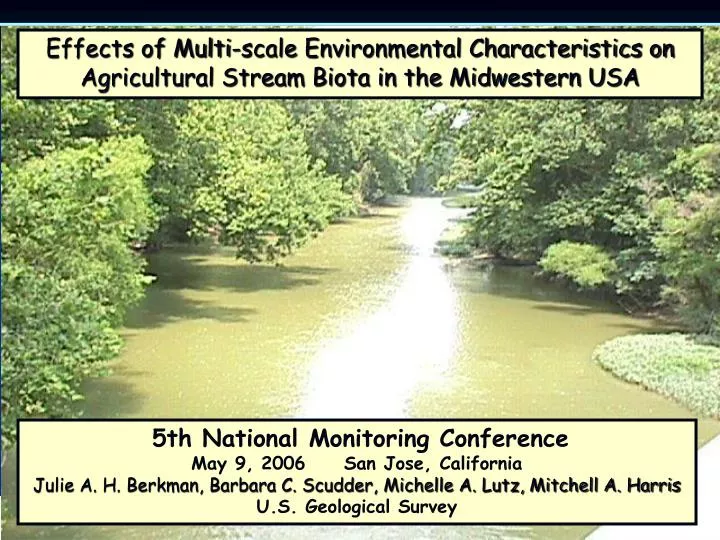
Effects of Multi-scale Environmental Characteristics on Agricultural Stream Biota in the Midwestern USA. 5th National Monitoring Conference May 9, 2006 San Jose, California Julie A. H. Berkman, Barbara C. Scudder, Michelle A. Lutz, Mitchell A. Harris U.S. Geological Survey. Outline.

E N D
Effects of Multi-scale Environmental Characteristics on Agricultural Stream Biota in the Midwestern USA 5th National Monitoring Conference May 9, 2006 San Jose, California Julie A. H. Berkman, Barbara C. Scudder, Michelle A. Lutz, Mitchell A. HarrisU.S. Geological Survey
Outline • Purpose • Overall approach • Geographical setting and site selection • Data collection and analysis: • What is meant by multiple scales? • Which environmental characteristics were used as variables? • What aspects of the biological assemblages were used? • How were environmental and biological data brought together? • What are our results at multiple spatial scales? • Relating BMPs and biological-assemblage responses
Purpose • Evaluate responses of stream biological assemblages to environmental variables across multiple-scales in agricultural watersheds • Identify the strongest relations between biological and environmental data that can be applied to assessing water-quality improvements in agricultural watersheds throughout the Midwest • Assess which physical variables are the best focus for improvements in water quality through agricultural BMPs, for which we spend about $4,000,000,000 per year nationally (Shields et al., 2006)
ND MN WI MI IA IN OH IL
Steps in Assessment • Organize assessment approach • Identify agricultural practices for improvement of water quality • Develop assessment endpoints • Define geographic scope • Build scientific foundation for assessment • Evaluate biological assemblages in relation to environmental variables at multiple spatial scales • Identify relations between biota and agricultural BMPs • Develop a conceptual model or index for measuring improvement due to specific agricultural BMPs • Verify • Calibrate and validate • Publicize—Outreach and implementation
What is meant by scale? Why does scale matter in monitoring streams? Segment Reach Basin Sample collection substrate
Reach Segment Watershed Photo of watershed by Mitch Harris
Segment margin “Riparian buffer” 15 m from bankfull • Percent land cover length • Average land cover length • Percent disturbed vs. natural • Number of fragments
Algae Photos by Rich Frehs Photo by Robert Sheath
Invertebrates Photo by Debby Murphy
Fish Photos by Mac Albin
PRIMER BioEnv analysis Samples Species percent abundance Bray-Curtis Rank correlation ps Abiotic variables Euclidean ps = An index of agreement of the two triangular matrices
An example of the results of reach variables & algae assemblages Best resultsout of 28 reach variables rank correlation ps =0.232 - 0.240 • Average stream velocity • Percent riffles • Percent fine silty substrate • Percent stream bank erosion • Percent 50-m buffer in woody vegetation • Percent bank covered by vegetation
Summary of correlations between biological assemblages and environmental variables at each physical scale With n=86, the 5% two-tailed significance level occurs when >0.210 1% two-tailed significance level occurs when >0.275
Summary of correlations between biological assemblages and environmental variables at each physical scale
Steps in Assessment • Organize the assessment approach • Identify agricultural practices for improvement of water quality • Develop assessment endpoints • Define geographic scope • Build a scientific foundation for the assessment • Evaluate biological assemblages in relation to environmental variables at multiple spatial scales • Identify relations between biota and agricultural BMPs • Develop a conceptual model or index for measuring improvement due to specific agricultural BMPs • Verify • Calibrate and validate • Publicize—Outreach and implementation
Bank stabilization (percent bank erosion) Bank vegetative cover Riparian buffer (avg. length of undisturbed buffer/km) Woody vegetation, 50 m Reduce sediment runoff (percent fine substrate) Algae and Invertebrates Algae, Invert., and Fish Fish Algae and Invertebrates Algae* (from rock substrates) Agricultural BMP At which scale are the BMPs being applied? At which scale should the effects be assessed? Biological response
Conservation Effects Assessment Project www.nrcs.usda.gov/technical/nri/ceap
Summary • The responses of stream biological assemblages to environmental characteristics across multiple scales revealed the importance of the larger scale watershed variables for all three groups, but especially the fish. • The strongest relations between biological and environmental data were identified and whether the biological assemblage had positive or negative response. For example sensitive fish, cobble fish, and the alga Achnanthidium minutissimum (Kützing) Czarnecki were all positively associated with stream velocity, percent riffles, and bank vegetative cover while tolerant algae and invertebtrates, as well as omnivorous fish were negatively correlated with these features. • Physical variables that can be managed through Best Management Practices such as bank vegetative cover and woody vegetation in riparian buffer at the reach scale and undisturbed buffer at the segment scale, were matched with biota that could be used to assess improvements in water quality.
Next steps are to identify • Relations between biota and agricultural BMPs • Scale at which the BMPs are applied, and • Which biologic endpoints would be best for assessing water-quality improvements in agricultural watersheds throughout the Midwest.
Thank you Coauthors: Barbara Scudder, Michelle Lutz, and Mitchell Harris Others who have provided valued assistance: USGS Wisconsin WSC Amanda Bell Faith Fitzpatrick James Kennedy Jana Stewart USGS National Research Program, Menlo Park, CA James L. Carter USGS Nebraska Water Science Center Michaela Johnson
Julie A. Hambrook Berkman, Ph.D. U.S. Geological Survey 6480 Doubletree Ave. Columbus, OH 43229-1111 jberkman@usgs.gov 614-430-7730 Barbara C. Scudder U.S. Geological Survey 8505 Research Way Middleton, WI 53562-3581 bscudder@usgs.gov 608-821-3832 For more information on this study contact: