Download
1 / 22
220 likes | 318 Views
ME - 495 Mechanical and Thermal Systems Lab Fall 2011 Chapter 3: Assessing and Presenting Experimental Data Professor: Sam Kassegne, PhD, PE. Lecture Covers. Terminologies (error, precision, resolution, etc) Statistical Theory Based on Population

E N D
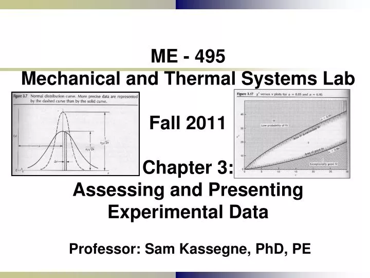
ME - 495 Mechanical and Thermal Systems LabFall 2011Chapter 3: Assessing and Presenting Experimental Data Professor: Sam Kassegne, PhD, PE
Lecture Covers • Terminologies (error, precision, resolution, etc) • Statistical Theory Based on Population • Statistical Theory Based on Sample (student ‘t’, Chi squared, etc) • Homework Problems
1) TERMINOLOGIES ERRORS • Error = ε = Xm – Xtrue: • Difference between measured and true values • Can never be calculated exactly • Bias/Systematic errors: errors that occur the same way each time a measurement is taken • Cannot be treated using statistics • Commonly a zero offset or scale error • Precision/Random errors: different for each measurement but average to zero
COMBINED ERROR Bias error > typical precision error typical precision error > bias error
CLASSIFICATION OF ERROR • Bias or systematic error • Calibration errors • Certain consistently recurring human errors • Certain errors caused by defective equipment • Loading errors • Limitations of system resolution • Precision or random error • Human error • Errors caused by disturbance of the equipment • Errors caused by fluctuating experimental conditions • Errors derived from insufficient measuring-system sensitivity
OTHER ERRORS • Illegitimate error • Blunders and mistakes during experimentation • Computational errors in data reduction • Errors that are sometimes bias and sometimes precision error • Errors from instrument backlash, friction, hysteresis • Errors from calibration drift, variation in test and environmental conditions
Introduction to UNCERTAINTY • Uncertainty: • Where: • Bx = bias uncertainty • Px = precision uncertainty
ESTIMATING PRECISION UNCERTAINTY • Distribution of error: probability that an error of given size will occur • Population: finite or infinite group from which samples are drawn • Sample: limited set of measurements • Gaussian or Normal Distribution (bell curve) • Probable difference/Confidence Interval: • Estimate of precision uncertainty of the measured sample
SAMPLE vs. POPULATION • A sample has a defined number of members (n) • A population may have: • (n) members or may be infinite • A sample is randomly taken from a population of indefinite size
PROBABILITY DISTRIBUTIONS • Histogram (Tossed Dice) • Distribution Types: • Gaussian (standard) • Students t-distribution • χ2 distribution (lower right)
2) THEORY BASED ON POPULATION • Probability Density Function (PDF) • Describes random precision error of sampling • Probability = area under curve
GAUSSIAN DISTRIBUTION • For Gaussian Distribution: • x = magnitude of particular measurement • μ = mean value of entire population • σ = standard deviation of entire population • μ Xavg = (x1+x2+…+xn)/n for large n • For a measurement (x) the deviation (d) d = x - μ
GAUSSIAN DISTRIBUTION (ctd.) • σ = standard deviation • Probability estimates • Standard curve
Probability • Question: • What is the area under the curve between z = -1.43 and z=1.43? • What range of z will contain 90% of the data?
3) THEORY BASED ON SAMPLE • Mean • Standard Deviation
Useful Terms in Theory Based on Samples Central Limit Theorem - For large number of n for a given number of samples, the distribution of the mean values is Gaussian.Eq 1. Confidence Interval (c%) - used to indicate the reliability of an estimate. How likely the interval is to contain the parameter is determined by the confidence level. For a population with unknown mean m and known standard deviation s, a confidence interval for the population mean, based on a simple random sample of size n is: Eq 2. Remember that: Eq 3 & Eq 4.
A) Student’s t-statistic • Useful for estimating confidence interval for small samples (n << 30) • Assumes the underlying population satisfies the Gaussian distribution • Considers the distribution of a quantity ‘t’ for a specific confidence interval
Student’s t-statistic • Probability for the t-statistic approaches Gaussian as n infinity • t-statistic eliminates probable outliers and what remains must center around the true value n = n-1 n is called the degree of freedom)
Student’s t-statistic • Example 3.6 on pg 74 • designates the area (hence probability) outside a specified value of ta. Conversely,the probability that a given value will lie inside of the limits ta is 1-a. n = 14, = 1.009 oz. Sx = 0.04178, n = 13. From Table 3.6, t0.025,13 = 2.160 two sided interval = +/-t0.025,13Sx/sqrt(n) = +/- 0.02412. m = 1.009 +/- 0.024 oz with CI of 95%
B) CHI SQUARED TEST * The χ2 test measures ‘goodness of fit’ * Tests the probability that a sample of data is or is not normally distributed. total area under curve = unity. Curve starts at chi^2 = 0 The curve is not symmetrical. As number of data increases, it becomes similar to normal distribution.
CHI SQUARED TEST – measures the ‘goodness of fit’ The χ2 goodness of fit test • Oi = the number of observed data in a bin • Ei = the number of expected data in a bin • N = the number of data bins, or “class intervals” • = degrees of freedom=1- number of bins Large discrepancy between Oi and Ei
CHI SQUARED EXAMPLE • For a group of 50 trees on a set area of land, to determine if the trees prefer dry soil we examine the following: • If 50% of the land is dry, 30% is moist, and 20% is wet, then if there were no preference, we would expect: • 25 trees on dry soil; 15 on moist; and 10 on wet • If actually: 40 on dry; 8 on moist; 2 on wet • 40-25=15; 152/25=9 | 8-15=7; 72/15=3.2 | 2-10=8; 82/10=6.4 • χ2= (9+3.2+6.4)= 18.6 • Examining the previous graph it is shown that it is extremely unlikely that there is no soil preference, as our Chi squared value falls far above the questionable probability (Note that bin-size, n = 3; nu = 2)