Download
1 / 20
210 likes | 365 Views
Spatial-Temporal Modelling of Extreme Rainfall. Climate Adaptation Flagship. Mark Palmer and Carmen Chan 11 th IMSC July 2010. Outline of talk. What we wanted to do What data did we have What data did we use How we got the most out of it Borrowing strength BHM’s Combining data

E N D
Spatial-Temporal Modelling of Extreme Rainfall Climate Adaptation Flagship Mark Palmer and Carmen Chan 11th IMSC July 2010
Outline of talk • What we wanted to do • What data did we have • What data did we use • How we got the most out of it • Borrowing strength BHM’s • Combining data • Squeezing data Colleagues: Aloke Phatak, Eddy Campbell, Bryson Bates, Santosh Aryal, Neil Viney, Carmen Chan, Yun Li 11th IMSC
What did we want to do • Describe the characteristics of extreme rainfall over a relatively large area, which includes • both gauged and ungauged sites • Model the tails of the rainfall distribution • Be able to estimate return levels for various periods • Be able to calculate Intensity-Duration-Functions (IDF) curves • Be able to calculate Depth-Area (DA) and Areal-Reduction-Factors (ARF) curves 11th IMSC
Return Levels, Return Periods • The return period T, for a given duration(say 24 hours) and intensity i(d), is the average time interval between exceedance of the value i(d) • ie the Return Period is the reciprocal of the probability of exceedance of that event. • Corresponding to the return period T is the return level i(d) “there is no universally agreed definition of this quantity, but one definition is that it is the level exceeded in any one year with probability 1/N. The less precise definition is the level which is exceeded ‘once in N years’ is problematical if there is a trend in the process (for example)’” Smith (2001) 11th IMSC
Intensity Duration Frequency (IDF) Curves • Intensity Duration Frequency • X-axis duration • Y-axis intensity • Each line corresponds to a fixed return period 11th IMSC
What data do we have Commonly • Daily data (measured from >9am to 9am the following day) • Pluvio data • essentially continuous measurements), though generally discretised to small (say 5 minute) intervals • can then aggregate this data for any duration of interest, using a sliding window • Issues • Quality • Spatial sparsity • Temporal sparsity, gaps • Untagged accumulations • homogenization 11th IMSC
Apparent embarrassment of riches 11th IMSC
What data do we keep • The BoM high quality data set is too small (particularly spatially) • The minimal requirement is for seasonal data (eg summer winter) that we know the maximal value of! • Can have short time series • Can have temporal gaps • If there are problems with summer data, might still be able to use winter data for that year (and vice versa) • Any bit of ‘information’ in the data is potentially useful (better than completely omitting it) 11th IMSC
How to get the most out of it • Develop a BHM with both spatial and temporal components • Allows us to borrow strength (ie sites that are “close” together should have similar characteristics • Anticipate that small proportions of ‘unusual’ sites or rainfall measurements will be ‘smoothed’ over, rather than having an undue influence on the analysis 11th IMSC
Based on a remarkable distributional result: Central to the statistical modelling of extreme values is the generalized extreme value (GEV) distribution. • If represents the maximum of a sequence of independent random variables (say daily rainfall over a year), then the distribution of (the yearly maximum rainfall), is given by • a very general result • Its relationship to modelling extremes is analogous to the use of the Normal distribution for modelling means or sums of random variables, regardless of their parent distribution (CLT). • the parameters the location, scale and shape parameters characterise the distribution of the extremes • we describe changes in extremes by changes in these parameters 11th IMSC
At-site model • Generally • Use a Generalised Extreme Value (GEV) distribution to characterise extreme rainfall at a site • Assume that changes in climate are reflected by changes in the GEV parameters at a site • Assume these GEV’s vary smoothly spatially (Convolution kernel approach, Higdon, Sanso etc) • Take block maxima approach (ie just use the largest value from each season, year by year) • Doesnt this waste data? • What about Generalised Pareto (GPD) approach (why not) • So, what can we do to maximise information 11th IMSC
Getting most out of available data • Build a BHM to borrow strength • Use r-order statistics (smaller standard errors, better fit) • Reparameterise location to dispersion coefficient (Koutsiyannis, Buishand) • Combine over durations (Koutsiyannis et al., 1998) • Constant shape parameter (Nadarajah, Anderson, and J.A. Tawn (1998) • Constant dispersion coefficient (empirically observed) • Model scale parameter over durations (ie now have 5 parameters per site) • ‘correct’ daily GEV to 24 hour basis. • The maxima from 24 hour aggregated data will be larger than the maxima of daily data [Robinson and Tawn, 2000], so estimate the extremal index, which is used to adjust the location and scale parameters of the GEV for the daily data to make it comparable with GEVs estimated from 24 hour data (the shape parameter remains unchanged 11th IMSC
Example of various durations:modelled scale parameter 11th IMSC
Spatial model ‘between’ covariates eg elevation ‘within’ covariates eg ocean heat GEV parameters ‘within’ covariates coefficients Rainfall Example: BHM,fitted by MCMC Di-graph representation of the Spatial-Temporal model for extreme rainfall 11th IMSC
Results: Spatial plots of parameters • Model the scale parameter as a linear function of OHC Fitted surfaces of GEV parameters from MCMC sampling; (a) dispersion coefficient, (b) scale (intercept) parameter, (c) linear ocean heat anomaly coefficient for modelling scale parameter, (d) log(shape) parameter, (e) theta parameter, (f) eta parameter 11th IMSC
Results: Return Level plots • Return level plots Differenced return levels surfaces (2003 – 1953) for a fifty year return period (a), and associated standard error surface (b). 11th IMSC
Results: IDF Curves Sample of IDF curves for the pluviograph site 566038, for a 50 year return period (Ocean heat anomaly = 0, i.e. effectively the historical long term average), drawn from the MCMC procedure, median value indicated by solid black line, broken lines indicate 0.025 and 0.975 quantiles. • IDF curves 11th IMSC
Conclusions: • Build a BHM to borrow strength, and combine many sources of data • Use r-order statistics • Combine over durations • Model scale parameter over durations • ‘correct’ daily GEV to 24 hour basis • Reparameterise location to dispersion coefficient is useful • Would like to say something about the extremes of areal rainfall using this approach, but: Warning: • Assumption of conditional independence between sites after spatial modelling of GEV parameters is wrong, • try sampling from it • need to model this, eg Copulas, max-stable approach (composite likelihoods) 11th IMSC
Mark Palmer Phone: +61 8 9333 6293 Email: mark.palmer@csiro.au Web: www.csiro.au/cmis Thank you Contact UsPhone: 1300 363 400 or +61 3 9545 2176Email: Enquiries@csiro.au Web: www.csiro.au
Koutsiyannis reparameterization Reparameterise location to dispersion coefficient • properties of the GEV might give some help 11th IMSC