Calculating Entropy Change

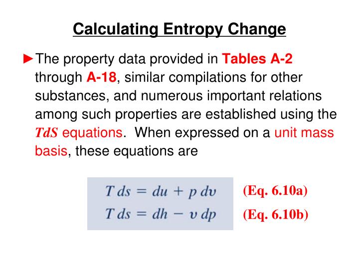
1. Calculating Entropy Change • The property data provided in Tables A-2 through A-18, similar compilations for other substances, and numerous important relations among such properties are established using the TdS equations. When expressed on a unit mass basis, these equations are (Eq. 6.10a) (Eq. 6.10b)

2. Defining Entropy Change • Recalling (from Sec. 1.3.3) that a quantity is a property if, and only if, its change in value between two states is independent of the process linking the two states, we conclude that the integral represents the change in some property of the system. • We call this property entropy and represent it by S. The change in entropy is (Eq. 6.2a) where the subscript “int rev” signals that the integral is carried out for any internally reversible process linking states 1 and 2.

3. (Eq. 6.23) where the subscript b indicates the integral is evaluated at the system boundary. (Eq. 6.24)

4. Assume pure simple compression system undergoing internally reversible process

5. Assume pure simple compression system undergoing internally reversible process (Eq. 6.10a) (Eq. 6.10b)

6. Calculating Entropy Change • As an application, consider a change in phase from saturated liquid to saturated vapor at constant pressure. • Since pressure is constant, Eq. 6.10b reduces to give • Then, because temperature is also constant during the phase change (Eq. 6.12) This relationship is applied in property tables for tabulating (sg – sf) from known values of (hg – hf).

7. Calculating Entropy Change • For example, consider water vapor at 100oC (373.15 K). From Table A-2, (hg – hf) =2257.1 kJ/kg. Thus (sg – sf) = (2257.1 kJ/kg)/373.15 K = 6.049 kJ/kg∙K which agrees with the value from Table A-2, as expected. • Next, the TdS equations are applied to two additional cases: substances modeled as incompressible and gases modeled as ideal gases.

8. (Eq. 6.13) Calculating Entropy Change of an Incompressible Substance • The incompressible substance model assumes the specific volume is constant and specific internal energy depends solely on temperature: u = u(T). Thus, du = c(T)dT, where c denotes specific heat. • With these relations, Eq. 6.10a reduces to give • On integration, the change in specific entropy is • When the specific heat is constant

9. Calculating Entropy Change of an Ideal Gas • The ideal gas model assumes pressure, specific volume and temperature are related by pv = RT. Also, specific internal energy and specific enthalpy each depend solely on temperature: u = u(T), h = h(T), giving du=cvdT and dh=cpdT, respectively. • Using these relations and integrating, the TdS equations give, respectively (Eq. 6.17) (Eq. 6.18)

10. Calculating Entropy Change of an Ideal Gas • Since these particular equations give entropy change on a unit of mass basis, the constant R is determined from • Since cv and cp are functions of temperature for ideal gases, such functional relations are required to perform the integration of the first term on the right of Eqs. 6.17 and 6.18. • For several gases modeled as ideal gases, including air, CO2, CO, O2, N2, and water vapor, the evaluation of entropy change can be reduced to aconvenient tabular approach using the variable so defined by (Eq. 6.19) whereT'is an arbitrary reference temperature.

11. For air, Tables A-22 and A-22E provide so in units of kJ/kg∙K and Btu/lb∙oR, respectively. For the other gases mentioned, Tables A-23 and A-23E provide in units of kJ/kmol∙K and Btu/lbmol∙oR, respectively. Calculating Entropy Change of an Ideal Gas • Using so, the integral term of Eq. 6.18 can be expressed as • Accordingly, Eq. 6.18 becomes (Eq. 6.20a) or on a per mole basis as (Eq. 6.20b)

12. Calculating Entropy Change of an Ideal Gas Example: Determine the change in specific entropy, in kJ/kg∙K, of air as an ideal gas undergoing a process from T1= 300 K, p1 = 1 bar to T2 = 1420 K, p2 = 5 bar. • From Table A-22, we get so1 = 1.70203 and so2 = 3.37901, each in kJ/kg∙K. Substituting into Eq. 6.20a Table A-22

13. Calculating Entropy Change of an Ideal Gas • Tables A-22 and A-22E provide additional data for air modeled as an ideal gas. These values, denoted by pr and vr, refer only to two states having the same specific entropy. This case has important applications, and is shown in the figure.

14. Calculating Entropy Change of an Ideal Gas • When s2 = s1, the following equation relates T1, T2, p1, and p2 (Eq. 6.41) (s1 = s2, air only) wherepr(T)is read from Table A-22 or A-22E, as appropriate. Table A-22

15. Calculating Entropy Change of an Ideal Gas • When s2 = s1, the following equation relates T1, T2, v1, and v2 (Eq. 6.42) (s1 = s2, air only) wherevr(T)is read from Table A-22 or A-22E, as appropriate. Table A-22

16. (Eq. 6.22) (Eq. 6.21) Entropy Change of an Ideal Gas Assuming Constant Specific Heats • When the specific heats cv and cp are assumed constant, Eqs. 6.17 and 6.18 reduce, respectively, to (Eq. 6.18) (Eq. 6.17) • These expressions have many applications. In particular, they can be applied to develop relations among T, p, and v at two states having the same specific entropy as shown in the figure.

17. Entropy Change of an Ideal GasAssuming Constant Specific Heats • Since s2 = s1, Eqs. 6.21 and 6.22 become • With the ideal gas relations wherekis the specific ratio • These equations can be solved, respectively, to give (Eq. 6.43) (Eq. 6.44) • Eliminating the temperature ratio gives (Eq. 6.45)

18. Calculating Entropy Change of an Ideal Gas Example: Air undergoes a process from T1= 620 K, p1 = 12 bar to a final state where s2 = s1, p2 = 1.4 bar. Employing the ideal gas model, determine the final temperature T2, in K. Solve using (a)pr data from Table A-22 and (b) a constant specific heat ratio k evaluated at 620 K from Table A-20: k = 1.374. Comment. (a) With Eq. 6.41 and pr(T1) = 18.36 from Table A-22 Interpolating in Table A-22, T2 = 339.7 K Table A-22

19. Calculating Entropy Change of an Ideal Gas (b) With Eq. 6.43 T2 = 345.5 K Comment: The approach of (a) accounts for variation of specific heat with temperature but the approach of (b) does not. With a k value more representative of the temperature interval, the value obtained in (b) using Eq. 6.43 would be in better agreement with that obtained in (a) with Eq. 6.41.

20. Isentropic Turbine Efficiency • For a turbine, the energy rate balance reduces to 1 2 • If the change in kinetic energy of flowing matter is negligible, ½(V12 – V22) drops out. • If the change in potential energy of flowing matter is negligible, g(z1 – z2) drops out. • If the heat transfer with surroundings is negligible, drops out. where the left side is work developed per unit of mass flowing.

21. Isentropic Turbine Efficiency • For a turbine, the entropy rate balance reduces to 1 2 • If the heat transfer with surroundings is negligible, drops out.

22. Isentropic Turbine Efficiency • Since the rate of entropy production cannot be negative, the only turbine exit states that can be attained in an adiabatic expansion are those with s2≥s1. This is shown on the Mollier diagram to the right. • The state labeled 2s on the figure would be attained only in an isentropic expansion from the inlet state to the specified exit pressure – that is, 2s would be attained only in the absence of internal irreversibilities. By inspection of the figure, the maximum theoretical value for the turbine work per unit of mass flowing is developed in such an internally reversible, adiabatic expansion:

23. Isentropic Turbine Efficiency • The isentropic turbine efficiency is the ratio of the actual turbine work to the maximum theoretical work, each per unit of mass flowing: (Eq. 6.46)

24. Isentropic Turbine Efficiency Example: Water vapor enters a turbine at p1= 5 bar, T1= 320oC and exits at p2 = 1 bar. The work developed is measured as 271 kJ per kgof water vapor flowing. Applying Eq. 6.46, determine the isentropic turbine efficiency. 1 2 • From Table A-4, h1 = 3105.6 kJ/kg, s1 = 7.5308 kJ/kg. With s2s = s1, interpolation in Table A-4 at a pressure of 1 bar gives h2s = 2743.0 kJ/kg. Substituting values into Eq. 6.46

25. Isentropic Compressor and Pump Efficiencies 1 • For a compressor the energy rate balance reduces to 2 • If the change in kinetic energy of flowing matter is negligible, ½(V12 – V22) drops out. • If the change in potential energy of flowing matter is negligible, g(z1 – z2) drops out. • If the heat transfer with surroundings is negligible, drops out. where the left side is workinput per unit of mass flowing.

26. Isentropic Compressor and Pump Efficiencies 1 • For a compressor the entropy rate balance reduces to 2 • If the heat transfer with surroundings is negligible, drops out.

27. Isentropic Compressor and Pump Efficiencies • Since the rate of entropy production cannot be negative, the only compressor exit states that can be attained in an adiabatic compression are those with s2≥s1. This is shown on the Mollier diagram to the right. • The state labeled 2s on the figure would be attained only in an isentropic compression from the inlet state to the specified exit pressure – that is, state 2s would be attained only in the absence of internal irreversibilities. By inspection of the figure, the minimum theoretical value for the compressor work input per unit of mass flowing is for such an internally reversible, adiabatic compression:

28. Isentropic Compressor and Pump Efficiencies • The isentropic compressor efficiency is the ratio of the minimum theoretical work input to the actual work input, each per unit of mass flowing: (Eq. 6.48) • An isentropic pump efficiency is defined similarly.

29. The objective is to introduce expressions for the heat transfer rate and work rate in the absence of internal irreversibilities. The resulting expressions have important applications. Heat Transfer and Work in Internally Reversible Steady-State Flow Processes • Consider a one-inlet, one-exit control volume at steady state: • Compressors, pumps, and other devices commonly encountered in engineering practice are included in this class of control volumes.

30. Heat Transfer and Work in Internally Reversible Steady-State Flow Processes • In agreement with the discussion of energy transfer by heat to a closed system during an internally reversible process (Sec. 6.6.1), in the present application we have (Eq. 6.49) where the subscript “int rev” signals that the expression applies only in the absence of internal irreversibilities. • As shown by the figure, when the states visited by a unit mass passing from inlet to exit without internal irreversibilities are described by a curve on a T-sdiagram, the heat transfer per unit of mass flowing is represented by the area under the curve.

31. Heat Transfer and Work in Internally Reversible Steady-State Flow Processes • Neglecting kinetic and potential energy effects, an energy rate balance for the control volume reduces to • With Eq. 6.49, this becomes (1) • Since internal irreversibilities are assumed absent, each unit of mass visits a sequence of equilibrium states as it passes from inlet to exit. Entropy, enthalpy, and pressure changes are therefore related by the TdS equation, Eq. 6.10b:

32. Heat Transfer and Work in Internally Reversible Steady-State Flow Processes • Integrating from inlet to exit: • With this relation Eq. (1) becomes (Eq. 6.51b) • If the specific volume remains approximately constant, as in many applications with liquids, Eq. 6.51b becomes (Eq. 6.51c) This is applied in the discussion of vapor power cycles in Chapter 8.

33. Heat Transfer and Work in Internally Reversible Steady-State Flow Processes • As shown by the figure, when the states visited by a unit mass passing from inlet to exit without internal irreversibilities are described by a curve on a p-v diagram, the magnitude of ∫vdp is shown by the area behind the curve.

34. Heat Transfer and Work in Internally Reversible Steady-State Flow Processes Example: A compressor operates at steady state with natural gas entering at at p1,v1. The gas undergoes a polytropic process described by pv = constant and exits at a higher pressure, p2. 1 2 (a) Ignoring kinetic and potential energy effects, evaluate the work per unit of mass flowing. (b) If internal irreversibilities were present, would the magnitude of the work per unit of mass flowing be less than, the same as, or greater than determined in part (a)?

35. Heat Transfer and Work in Internally Reversible Steady-State Flow Processes (a) With pv= constant, Eq. 6.51b gives The minus sign indicates that the compressor requires a work input. (b) Left for class discussion.

37. Second Law of ThermodynamicsAlternative Statements • Clausius Statement • Kelvin-Planck Statement • Entropy Statement There is no simple statement that captures all aspects of the second law. Several alternativeformulations of the second law are found in the technical literature. Three prominent ones are:

38. The Kelvin temperature is defined so that (Eq. 5.7) Kelvin Temperature Scale Consider systems undergoing a power cycle and a refrigeration or heat pump cycle, each while exchanging energy by heat transfer with hot and cold reservoirs:

39. Example: Power Cycle Analysis A system undergoes a power cycle while receiving 1000 kJ by heat transfer from a thermal reservoir at a temperature of 500 K and discharging 600 kJ by heat transfer to a thermal reservoir at (a) 200 K, (b) 300 K, (c) 400 K. For each case, determine whether the cycle operatesirreversibly, operatesreversibly, or is impossible. Solution: To determine the nature of the cycle, compare actual cycle performance (h) to maximum theoretical cycle performance (hmax) calculated from Eq. 5.9

40. Clausius Inequality • The Clausius inequality considered next provides the basis for developing the entropy concept in Chapter 6. • The Clausius inequality is applicable to any cycle without regard for the body, or bodies, from which the system undergoing a cycle receives energy by heat transfer or to which the system rejects energy by heat transfer. Such bodies need not be thermal reservoirs.

41. ∫ (Eq. 5.13) where ∫ indicates integral is to be performed over all parts of the boundary and over the entire cycle. b subscript indicates integrand is evaluated at the boundary of the system executing the cycle. Clausius Inequality • The Clausius inequality is developed from the Kelvin-Planck statement of the second law and can be expressed as:

42. Example: Use of Clausius Inequality A system undergoes a cycle while receiving 1000 kJ by heat transfer at a temperature of 500 K and discharging 600 kJ by heat transfer at (a) 200 K, (b) 300 K, (c) 400 K. Using Eqs. 5.13 and 5.14, what is the nature of the cycle in each of these cases? Solution: To determine the nature of the cycle, perform the cyclic integralof Eq. 5.13 to each case and apply Eq. 5.14 todraw a conclusion about the nature of each cycle.

43. ∫ Example: Use of Clausius Inequality Applying Eq. 5.13 to each cycle:

44. Defining Entropy Change • Recalling (from Sec. 1.3.3) that a quantity is a property if, and only if, its change in value between two states is independent of the process linking the two states, we conclude that the integral represents the change in some property of the system. • We call this property entropy and represent it by S. The change in entropy is (Eq. 6.2a) where the subscript “int rev” signals that the integral is carried out for any internally reversible process linking states 1 and 2.

45. Entropy Facts • Entropy is an extensive property. • Like any other extensive property, the change in entropy can be positive, negative, or zero: • By inspection of Eq. 6.2a, units for entropyS are kJ/K and Btu/oR. • Units forspecific entropys are kJ/kg∙K and Btu/lb∙oR.

46. Entropy Facts • For problem solving, specific entropy values are provided in Tables A-2 through A-18. Values for specific entropy are obtained from these tables using the same procedures as for specific volume, internal energy, and enthalpy, including use of (Eq. 6.4) for two-phase liquid-vapor mixtures, and (Eq. 6.5) for liquid water, each of which is similar in form to expressions introduced in Chap. 3 for evaluating v, u, and h.

47. Entropy and Heat Transfer • In an internally reversible, adiabatic process (no heat transfer), entropy remains constant. Such a constant-entropy process is called an isentropic process. • On rearrangement, Eq. 6.2b gives Integrating from state 1 to state 2, (Eq. 6.23)

48. Entropy and Heat Transfer From this it follows that an energy transfer by heat to a closed system during an internally reversible process is represented by an area on a temperature-entropy diagram:

49. Entropy Balance for Closed Systems • The entropy balance for closed systems can be developed using the Clausius inequality expressed as Eq. 5.13 and the defining equation for entropy change, Eq. 6.2a. The result is where the subscript b indicates the integral is evaluated at the system boundary. (Eq. 6.24) • In accord with the interpretation of scycle in the Clausius inequality, Eq. 5.14, the value of s in Eq. 6.24 adheres to the following interpretation = 0 (no irreversibilities present within the system) > 0 (irreversibilities present within the system) < 0 (impossible) s:

50. 2 1 Entropy Balance for Closed Systems Example: One kg of water vapor contained within a piston-cylinder assembly, initially at 5 bar, 400oC, undergoes an adiabatic expansion to a state where pressure is 1 bar and the temperature is (a)200oC, (b)100oC. Using the entropy balance, determine the nature of the process in each case. Boundary • Since the expansion occurs adiabatically, Eq. 6.24 reduces to give 0 → m(s2 – s1) = s (1) wherem = 1 kg and Table A-4 gives s1 = 7.7938 kJ/kg∙K.