Download
1 / 27
270 likes | 396 Views
Introduction into STATA III: Graphs and Regressions. Prof. Dr. Herbert Brücker University of Bamberg Seminar “Migration and the Labour Market” June 27, 2013. 1 GRAPHS Present your data graphically

E N D
Introduction into STATA III: Graphs and Regressions Prof. Dr. Herbert Brücker University of Bamberg Seminar “Migration and the Labour Market” June 27, 2013
1 GRAPHS • Present your data graphically • It is usually helpful if you present the main information /vairables in your data set graphically • There are many graphical commands, use the Graphicsmenue • the simplest way is to show the development of your variable(s) over time • Syntax: • graph twoway line [variable1] [variable2] if … • graph twoway line wqjt year if ed==1 & ex == 1 • This produces a two-dimensional variable with the wage on the vertical and the year on the horizontal axis for education group 1 and experience group 1
GRAPHS: Two Y-axes • Two axes: It might be useful to display two variables in different y-axes with different scales (e.g. wages and migration rates) • Syntax: • graph (twoway line [variable1] [variable2], yaxis(1)) (twoway line [variable3] [variable2], yaxis(2)) if … • graph (twoway line wqjt year, yaxis(1)) (twoway line mqjt year, yaxis(2)) if ed==1 & ex == 1 • This produces a two-dimensional graph with the wage on the first vertical axis (y1) and the migration rate on the second vertical axis (y2)
GRAPHS: Scatter plots (I/II) • Scatter plots display the relations between two variables • Syntax: • graph twoway scatter [variable1] [variable2] if … • graph twoway scatter wqjtmqjt if ed==1 • This produces a two-dimensional scatter plot which shows the relation between the two variables
GRAPHS: Scatter plots (II/II) • You can also add a linear fitted line: • Syntax: • graph twoway scatter [variable1] [variable2] if …|| lfit [variable1] [variable2] if … • graph twoway scatter wqjtmqjt if ed==1|| lfitwqjtmqjt if ed==1
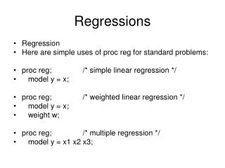
2 Running regressions • The standard OLS regression command in STATA is • Syntax • regress depvar [list of indepvar ] [if], [options] • e.g. regress ln_wijtmijt $D_i $D_j $D_t
The multivariate linear regression model The general econometric model: γi indicates the dependent (or: endogenous) variable x1i,ki exogenous variable, explaining the independent variable β0 constantorthe y-axisintercept (if x = 0) β1,2,k regressioncoefficientorparameterofregression εi residual, disturbanceterm
Running a regression model Globals ! Regressioncommand Dependentvariable Independentvariables
How to interpret the output of a regression variance of model degreesoffreedom 1. Observations2. fit of the model 3. F-Test 4. R-squared5. adjusted R-squared 6. Root Mean Standard Error β1 95% confidenceinterval β0 analysis of significance levels
Recall the Borjas (2003)-Modell • yijt = βmijt + si + xj + tt + (si ∙ xj) + (si ∙ tt) + (xj ∙ tt) + εijt • This model in STATA Syntax: • regress ln_wqjtmqjt $Di $Dj $Dt $Dij $Dit $Djt • where • ln_wqjt: dependent variable (log wage) • mqjt: migration share in educatipn-experience cell • $Di: global for education dummies • $Dj: global for experience dummies • $Dt: global for time dummies • $Dij: global for interaction education-experience dummies • $Dit: global for education-time interaction dummies • $Djt: global for experience-time interaction dummies
What is a global? • A global defines a vector of variables • Defining a global: • STATA Syntax: • global [global name] [variable1] [variable2] …[variablex] • global Di Ded1 Ded2 Ded3 • Using a global e.g. in a regression: • regress [depvariable] [other variable] [$global name] • regress ln_wqjtmqjt $Di • This is equivalent to: • regress ln_wqjtmqjt Ded1 Ded2 Ded3 • Thus, globals are useful shortcuts for lists (vectors) of variables.
An alternative to the Borjas (2003) model: • yijkt = βmijt + γk (zk∙ mijt) + si + xj + zk + tt + (si ∙ xj) + (si ∙ zk) + (xj ∙ zk) + (si ∙ tt) + (xj ∙ tt) + (zk ∙ tt) + εijt • where • zkis a dummy for foreigners (1 if foreigner, 0 if native) • γk is a coefficient, whichcapturesthe different impact on foreigners, • k (k= 0, 1) is a subscriptfornationality • Idea: theslopecoefficientγk issignificantly different fromzero, ifnatives andimmigrantsareimperfectsubstitutes in thelabourmarket. • Problem: Wehavetoreorganizethedataset such thatitdeliversthe wage andunemploymentrates etc. forforeignersand natives.
3 Panel Models • Very often you use panel models, i.e. models which have a group and time series dimension • There exist special estimators for this, e.g. fixed or random effects models • A fixed effects model is a model where you have a fixed (constant) effect for each individual/group. This is equivalent to a dummy variable for each group • A random effects model is a model where you have a random effect for each individual group, which is based on assumptions on the distribution of individual effects
Panel Models • Preparing data for Panel Models: • For running panel models STATA needs to identify the group(individual) and time series dimension • Therefore you need an index for each group and an index for each time period • Then use the tsset command to organize you dataset as a panel data set • Syntax: • tsset index year • where index is the group/individual index and year the time index
Running Regressions: Panel Models • Then you can use panel estimators, e.g. the xtreg estimator • Syntax • xtregressdepvar [list of indepvar ] [if], [options] • xtregressln_wijtm_ijt, fe • i.e. in the example we run a simple fixed effects panel regression model which is equivalent to include a dummy variable for each group (in this case education-experience group)
Running Regressions: Panel Models • There are other features of panel estimators which are helpful • Heteroscedasticity: • Heteroscedasticity: the variance is not constant, but varies across groups • xtpcse , p(h) corrects for heteroscedastic standard errors • xtgls , p(h) corrects coefficient and standard errors for panel heteroscedasticity, but may produce biased results depending on the group and time dimension of the panel • Note: p(h) after the comma is a so-called “option” in the STATA syntax
Running Regressions: Panel Models • Contemporary correlation across cross-sections • Contemporary correlation: the error terms are contemporarily correlated across cross-sections, e.g. due to macroeconomic disturbances • xtgls , p(c) corrects for contemporary correlation and panel heteroscedasticity, but may produce biased results depending on the group and time dimension of the panel.
Next Meeting • July 4! • Presentation: July 18 • Room RZ 01.02