Download

1 / 25
250 likes | 329 Views
ITCS 6163. Lecture 5. Indexing datacubes. Objective: speed queries up. Traditional databases (OLTP): B-Trees Time and space logarithmic to the amount of indexed keys. Dynamic, stable and exhibit good performance under updates. (But OLAP is not about updates….) Bitmaps :

E N D
ITCS 6163 Lecture 5
Indexing datacubes • Objective: speed queries up. • Traditional databases (OLTP): B-Trees • Time and space logarithmic to the amount of indexed keys. • Dynamic, stable and exhibit good performance under updates. (But OLAP is not about updates….) • Bitmaps: • Space efficient • Difficult to update (but we don’t care in DW). • Can effectively prune searches before looking at data.
R = (…., A,….., M) R (A) B8 B7 B6B5 B4 B3 B2 B1 B0 3 0 0 0 0 0 1 0 0 0 2 0 0 0 0 0 0 1 0 0 1 0 0 0 0 0 0 0 1 0 2 0 0 0 0 0 0 1 0 0 8 1 0 0 0 0 0 0 0 0 2 0 0 0 0 0 0 1 0 0 2 0 0 0 0 0 0 1 0 0 0 0 0 0 0 0 0 0 0 1 7 0 1 0 0 0 0 0 0 0 5 0 0 0 1 0 0 0 0 0 6 0 0 1 0 0 0 0 0 0 4 0 0 0 0 1 0 0 0 0 Bitmaps
Query optimization Consider a high-selectivity-factor query with predicates on two attributes. Query optimizer: builds plans (P1) Full relation scan (filter as you go). (P2) Index scan on the predicate with lower selectivity factor, followed by temporary relation scan, to filter out non-qualifying tuples, using the other predicate. (Works well if data is clustered on the first index key). (P3) Index scan for each predicate (separately), followed by merge of RID.
Index Pred1 Index Pred2 Blocks of data (P2) (P3) t1 tn t1 tn Tuple list1 Tuple list2 Pred. 2 Merged list answer Query optimization (continued)
Query optimization (continued) When using bitmap indexes (P3) can be an easy winner! CPU operations in bitmaps (AND, OR, XOR, etc.) are more efficient than regular RID merges: just apply the binary operations to the bitmaps (In B-trees, you would have to scan the two lists and select tuples in both -- merge operation--) Of course, you can build B-trees on the compound key, but we would need one for every compound predicate (exponential number of trees…).
Bitmap for a1 Bitmap for b2 Bitmap for a1 and b2 Bitmaps and predicates A = a1 AND B = b2 = AND
Tradeoffs Dimension cardinality small dense bitmaps Dimension cardinality large sparse bitmaps Compression (decompression)
Fact table Dimension table … a ... k … Prod. Bitmap for loc. Bitmap for prod Bitmap for prod Bitmap for type a Bitmap for type k Bitmap for loc. ….. ….. ….. Query strategy for Star joins Maintain join indexes between fact table and dimension tables
Bitmap for Bitmap for Bitmap for Bitmap for predicate Strategy example Aggregate all sales for products of location , or = OR OR
Star-Joins Select F.S, D1.A1, D2.A2, …. Dn.An from F,D1,D2,Dn where F.A1 = D1.A1 F.A2 = D2.A2 … F.An = Dn.An and D1.B1 = ‘c1’ D2.B2 = ‘p2’ …. Likely strategy: For each Di find suitable values of Ai such that Di.Bi = ‘xi’ (unless you have a bitmap index for Bi). Use bitmap index on Ai’ values to form a bitmap for related rows of F (OR-ing the bitmaps). At this stage, you have n such bitmaps, the result can be found AND-ing them.
Example Selectivity/predicate = 0.01 (predicates on the dimension tables) n predicates (statistically independent) Total selectivity = 10 -2n Facts table = 108 rows, n = 3, tuples in answer = 108/ 106 = 100 rows. In the worst case = 100 blocks… Still better than all the blocks in the relation (e.g., assuming 100 tuples/block, this would be 106 blocks!)
Design Space of Bitmap Indexes The basic bitmap design is called Value-list index. The focus there is on the columns. If we change the focus to the rows, the index becomes a set of attribute values (integers) in each tuple (row), that can be represented in a particular way. 5 0 0 0 1 0 0 0 0 0 We can encode this row in many ways...
Attribute value decomposition C = attribute cardinality Consider a value of the attribute, v, and a sequence of numbers <bn-1, bn-2 , …,b1>. Also, define bn = C / bi , then v can be decomposed into a sequence of n digits <vn, vn-1, vn-2 , …,v1> as follows: v = V1 = V2 b1 + v1 = V3(b2b1) + v2 b1 + v1 … n-1i-1 = vn ( bj) + …+ vi ( bj) + …+ v2b1 + v1 where vi = Vi mod bi and Vi = Vi-1/bi-1
< 7,7,5,3> 576/(7x7x5x3) = 576/735 = 0 | 576, 576/(7x5x3)=576/105=5|51 576 = 5 x (7x5x3)+51 Number systems How do you write 576 in: <2,2,2,2,2,2,2,2,2> 576 = 1 x 29 + 0 x 28 + 0 x 27 + 1 x 26 + 0 x 25 + 0 x 24 + 0 x 23 + 0 x 22+ 0 x 21 + 0 x 20 576/ 29 = 1 | 64, 64/ 28 = 0|64, 64/ 27 = 0|64, 64/ 26 = 1|0, 0/ 25 = 0|0, 0/ 24= 0|0, 0/ 23= 0|0, 0/ 22 = 0|0, 0/ 21 = 0|0, 0/ 20 = 0|0 <10,10,10> (decimal system!) 576 = 5 x 10 x 10 + 7 x 10 + 6 576/100 = 5 | 76 76/10 = 7 | 6 6 51/(5x3) = 51/15 = 3 | 6 6/3 =2 | 0 576 = 5 x (7x5x3) + 3 (5 x 3) + 16 576 = 5 x (7x 5 x 3) + 3 x (5 x 3 ) + 2 x (3)
R = (…., A,….., M) value-list index R (A) B8 B7 B6B5 B4 B3 B2 B1 B0 3 0 0 0 0 0 1 0 0 0 2 0 0 0 0 0 0 1 0 0 1 0 0 0 0 0 0 0 1 0 2 0 0 0 0 0 0 1 0 0 8 1 0 0 0 0 0 0 0 0 2 0 0 0 0 0 0 1 0 0 2 0 0 0 0 0 0 1 0 0 0 0 0 0 0 0 0 0 0 1 7 0 1 0 0 0 0 0 0 0 5 0 0 0 1 0 0 0 0 0 6 0 0 1 0 0 0 0 0 0 4 0 0 0 0 1 0 0 0 0 Bitmaps
sequence <3,3> value-list index (equality) R (A) B22B12B02 B21 B11 B01 3 (1x3+0) 0 1 0 0 0 1 2 0 0 1 1 0 0 1 0 0 1 0 1 0 2 0 0 1 1 0 0 8 1 0 0 1 0 0 2 0 0 1 1 0 0 2 0 0 1 1 0 0 0 0 0 1 0 0 1 7 1 0 0 0 1 0 5 0 1 0 1 0 0 6 1 0 0 0 0 1 4 0 1 0 0 1 0 Example
Encoding scheme Equality encoding: all bits to 0 except the one that corresponds to the value Range Encoding: the vi righmost bits to 0, the remaining to 1
Range encodingsingle component, base-9 R (A) B8 B7 B6B5 B4 B3 B2 B1 B0 3 1 1 1 1 1 1 0 0 0 2 1 1 1 1 1 1 1 0 0 1 1 1 1 1 1 1 1 1 0 8 1 0 0 0 0 0 0 0 0 0 1 1 1 1 1 1 1 1 1 7 1 1 0 0 0 0 0 0 0 5 1 1 1 1 0 0 0 0 0 6 1 1 1 0 0 0 0 0 0 4 1 1 1 1 1 0 0 0 0
sequence <3,3> value-list index(Equality) R (A) B22B12B02 B21 B11 B01 3 (1x3+0) 0 1 0 0 0 1 2 0 0 1 1 0 0 1 0 0 1 0 1 0 2 0 0 1 1 0 0 8 1 0 0 1 0 0 2 0 0 1 1 0 0 2 0 0 1 1 0 0 0 0 0 1 0 0 1 7 1 0 0 0 1 0 5 0 1 0 1 0 0 6 1 0 0 0 0 1 4 0 1 0 0 1 0 Example (revisited)
sequence <3,3> range-encoded index R (A) B12B02 B11 B01 3 1 0 1 1 2 1 1 0 0 1 1 1 1 0 2 1 1 0 0 8 0 0 0 0 2 1 1 0 0 2 1 1 0 0 0 1 1 1 1 7 0 0 1 0 5 1 0 0 0 6 0 0 1 1 4 1 0 1 0 Example
Design Space range equality ….
RangeEval Evaluates each range predicate by computing two bitmaps: BEQ bitmap and either BGT or BLT RangeEval-Opt uses only <= A < v is the same as A <= v-1 A > v is the same as Not( A <= v) A >= v is the same as Not (A <= v-1)