Download
1 / 27
270 likes | 384 Views
Model based Visualization of Cardiac Virtual Tissue. James Handley, Ken Brodlie – University of Leeds Richard Clayton – University of Sheffield. Tackling two Grand Challenge research questions: What causes heart disease How does a cancer form and grow?

E N D
Model based Visualization of Cardiac Virtual Tissue James Handley, Ken Brodlie – University of Leeds Richard Clayton – University of Sheffield
Tackling two Grand Challenge research questions: • What causes heart disease • How does a cancer form and grow? • Together these diseases cause 61% of all UK deaths.
Why model the heart? • Heart disease is an important health problem. • Worldwide, cardiovascular disease causes 19 million deaths annually, over 5 million between the ages of 30 and 69 years. • Spectrum of acquired and congenital heart disease, multiple disease mechanisms. • All disease mechanisms are difficult to study experimentally. • Heart is simpler (structurally and functionally) than other organs.
Ventricular Fibrillation – The Killer Normal rhythm Ventricular fibrillation How does it start? How can we stop it?
Cardiac Virtual Tissue Model cardiac tissue as a continuous excitable medium • Solve using finite difference grid. At each timestep • Compute dV due to diffusion • Compute dV due to dynamic response of cell membrane • Different models can be used; simplified and detailed • Update membrane voltage at each grid point
…but detailed models may have dozens of variables. The Visualization Challenge Standard Visualization techniques of 2D and 3D models use a single variable… Can we visualize the entire state of the heart model in a single image (or figure?)
Simplified and detailed models LuoRudy2 – 14 variable Fenton Karma 4 variable
The Visualization Challenge Impossible! (3+1) dimensional 14+ variate data cannot be perfectly visualized in a single picture on a (2+1) dimensional computer screen… .. but can we make at least a useful representation in a single image?
Reduce the data U V W D
x = 55, y = 91 Move into ‘Phase Space’ U V W Observation 1: 3 k x k images can be expressed as k x k points in 3-dimensional space
CVT data sets – Phase Space Visualization Using a 2D slice of Fenton Karma 3 variable CVT • Normal action potential propagation through homogeneous tissue • Re-entrant behaviour in heterogeneous tissue
Problem: This works for 3 variables – but generalisation for M variables is: M k x k images represented as k x k points in M-dimensional space How do we visualize M-dimensional space?? Phase Space Visualization
What does phase space look like for 14 variable Luo Rudy 2? • Look at 2D projections • Here are 13 phase space • representations of action potential • against other variables But.. can we get a single, composite picture - if possible, in the original space?
x = 55, y = 91 From ‘Phase Space’ to Image U V W Observation 2: M k x k images represented as 1 composite k x k image
We look first at two general techniques: Value according to density of points in that point’s neighbourhood of phase space Value according to position of point in phase space Assigning Value to a Point in Phase Space
x = 55, y = 91 x = 55, y = 91 According to Density - Form images using hyper-dimensional histograms using histogram sizes
x = 55, y = 91 x = 55, y = 91 According to Position - Form images using hyper-dimensional histograms using histogram IDs
Why not use knowledge of normal behaviour? Build a model of the expected locations of points in phase space For any simulation, visualize the difference from normal behaviour The value of a point then becomes the distance of the point from the model In this way abnormal points are highlighted to the greatest extent Model based Approach
Capture every point in M-dimensional phase space for simulation showing normal behaviour Typically this generates millions of points over time Model then decimated because: Many points co-located Distance calculation is expensive Any point removed is within ‘eps’ of point retained Typical reduction: 5 million to 500 Building the Point-based Model
Fenton Karma three variable model Model-based Representation Action Potential
Luo Rudy 2 fourteen variable model Action potential Model-based representation
New insight gained from moving to phase space – particularly for three variables Higher number of variables is challenging – but some merit in mapping M-dimensional phase space back to the image space by assigning phase space properties to pixels Approach will generalise to 3D models: 3 k x k x k volumes will map to k x k x k points in 3D phase space M k x k x k volumes will map to a composite k x k x k volume (via M-dimensional phase space) Conclusions