Download
1 / 36
370 likes | 608 Views
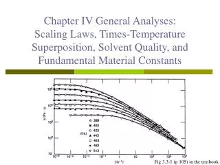
Chapter IV General Analyses: Scaling Laws, Times-Temperature Superposition, Solvent Quality, and Fundamental Material Constants. Fig 3.3-1 (p 105) in the textbook. Content of Chapter IV. Effects of Solvent Quality (pp. 139-143) Molecular-Weight Scaling Laws (pp.143-150)

E N D
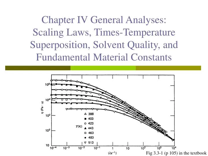
Chapter IV General Analyses: Scaling Laws, Times-Temperature Superposition, Solvent Quality, and Fundamental Material Constants Fig 3.3-1 (p 105) in the textbook
Content of Chapter IV • Effects of Solvent Quality (pp. 139-143) • Molecular-Weight Scaling Laws (pp.143-150) • Retrieval of Fundamental Material Constants • Time-Temperature Superposition: Application and Failure (pp. 105-108, 139-143) • Case Study
IV.1 Effects of Solvent Quality • Magnitude of intrinsic viscosity • -temperature & Solvent • Flow curve Fig 3.3-4 (p 107) in the textbook, or T. Kotaka et al., J. Chem. Phys. 45, 2770-2773 (1966).
IV.1 Effects of Solvent Quality • The solvent quality is an index describing the strength of polymer-solvent interactions. • This interaction strength is a function of chemical species of polymer & solvent molecules, temperature, and pressure. Scaling law of polymer size and molecular weight (<R2>end-to-end 1/2 ~ Mw).
IV.1 Effects of Solvent Quality poor good -temperature • Advantages of PMS: • High plasticized speed • Good temperature tolerance • Contamination resistance • Compatibility with other additives • Environment friendly N. Hadjichristidis et al., Macromolecules 24, 6725-6729 (1991).
IV.1 Effects of Solvent Quality The (temperature, weight fraction) phase diagram for the polystyrene-cyclohexane system for samples of Indicated molecular weight. S. Saeki et al, Macromolecules 6, 246-250(1973). TU: upper critical solution temperature TL: lower critical solution temperature
IV.1 Effects of Solvent Quality coil globule Poly(N-isopropylacrylamide) in water Mw = 4.45x10⁵ g/mol, c = 6.65x10⁻⁴ g/ml Mw = 1.00x10⁷ g/mol, c = 2.50x10⁻⁵ g/ml coil globule X. Wang et al., Macromolecules 31, 2972-2976 (1998). H. Yang et al., Polymer 44, 7175-7180 (2003).
IV.2.1 Molecular-Weight Dependence For linear polymer melts Mc (=2Me): critical molecular weight Me: entangled molecular weight Plot of constant + log 0 vs. constant + log M for nine different polymers. The two constants are different for each of the polymers, and the one appearing in the abscissa is proportional to concentration, which is constant for a given undiluted polymer. For each polymer the slopes of the left and right straight line regions are 1.0 and 3.4, respectively. [G. C. Berry and T. G. Fox, Adv. Polym. Sci. 5, 261-357 (1968).]
IV.2.2 Concentration Effect [cf. p109] An example of viscosity versus concentration plots for polystyrene (Mw=7.14106 g/mol) in benzene at 30 C. White circles: plot of sp / c vs. c; black circles: plot of (lnr)/c vs. c. (1) Zimm-Crothers viscometer (3.710-3 ~7.610-2 dyn/cm2); (2)Ubbelohde viscometer (8.67 dyn/cm2); (3)Ubbelohde viscometer (12.2 dyn/cm2). T. Kotaka et al., J. Chem. Phys. 45, 2770-2773 (1966).
IV.2.3 Impact of MolecularWeight Distribution H. Munstedt, J. Rheol. 24, 847-867 (1980)
IV.2.4 Molecular Architecture Linear PolymerStar PolymerPom-Pom Polymer polybutadienePolyisoprenePolyisoprene
IV.3 Retrieval of Fundamental Material Constants Newtonian Power law Zero-shear viscosity, 0 Fig 3.3-1 (p 105) in the textbook
IV.3 Retrieval of Fundamental Material Constants e ~ M0 d ~ M3 Storage modulus vs. frequency for narrow distribution polystyrene melts. Molecular weight ranges from Mw = 8.9x10³ r/mol (L9) to Mw = 5.8x10⁵ g/mol (L18). Theoretical results of (a) G(t) and (b) G’() for polymer melts. M. Doi and S. F. Edwards, The Theory of Polymer Dynamics, Oxford Science: New York (1986), pp 229-230.
IV.4 Time-Temperature Superposition • Time-temperature superposition holds for many polymer melts and solutions, as long as there are no phase transitions or other temperature-dependent structural changes in the liquid. • Time-temperature shifting is extremely useful in practical application, allows one to makeprediction of time-dependent material response.
IV.4 Time-Temperature Superposition WLF temperature shift parameters J. D. Ferry, Viscoelastic Properties of Polymers, 3rd ed., Wiley: New York (1980).
IV.4 Time-Temperature Superposition Master curves for the viscosity and first normal Stress coefficient as functions of shear rate for the Low-density polyethylene melt Non-Newtonian viscosity of a low-density polyethylene melt at several different temperature. Fig 3.3-1 and 3.3-2 (pp105-106) in the textbook.
IV.4 Time-Temperature Superposition A master curve of polystyrene-n-butyl benzene solutions. Molecular weights varied from 1.6x10⁵ to 2.4x10⁶ g/mol, concentration from 0.255 to 0.55 g/cm3, and temperature from 303 to 333 K. Fig 3.6-5 (p 146) in the textbook.
Chapter V Constitutive Equations and Modeling of Complex Flow Processing
Content of Chapter V • Models for Generalized Newtonian Fluids • Constitutive Equations for Generalized Linear Viscoelasticity • Objective Differential/Integral Constitutive Equations • Simulations of complex Flow Processing • Case Study
V.1 Models for Generalized Newtonian Fluids • In many industrial problems the most important feature of polymeric liquids is that their viscosity decrease markedly as the shear rate increases. • The generalized Newtonian model incorporates the idea of a shear-rate-dependent viscosity into the Newtonian constitute equation. • This generalized Newtonian model can not describe normal stress effects or time-dependent elastic effects.
V.1 Models for Generalized Newtonian Fluids • The Carreau-Yasuda model • The power-law model n < 1, shear-thinning (pesudoplastic) fluids n = 1 and m = , Newtonian fluids n > 1, shear-thickening (dilatant) fluids
V.1 Models for Generalized Newtonian Fluids • The Eyring model • The Bingham model • Other empirical functions in the generalized Newtonian fluid model (see Table 4.5-1, p 228 in the textbook)
V.2 Constitutive Equations for Generalized Linear Viscoelasticity • Goal: to introduce a equation that can describe some of the time-dependent motions of fluids under a flow with very small displacement gradients • Why do we concern the linear viscoelasticity (LVE) of fluids? (1) interrelatestructurewith the linear mechanical responses (2) proceed to the subject of nonlinear viscoelasticity • How to combine the idea of viscosity and elasticity into a single constitutive equation described various interesting elastic effects? shearing motion of a Newtonian fluid & Hookean solid
V.2 Constitutive Equations for Generalized Linear Viscoelasticity • The Maxwell model (concentrate solution or melt) Nature of flow Relaxation modulus, G(t) (pure polymer contribution) Nature of fluid
V.2 Constitutive Equations for Generalized Linear Viscoelasticity • The Jeffreys model (dilution solution) Relaxation modulus, G(t) (contribution of polymer and solvent)
V.3 Objective Differential/Integral Constitutive Equations • Quasi-linear model is obtained by reformulating the linear viscoelastic model. The convected Jeffreys model or Oldroyd’s fluid B • The convected Jeffreys model is derived from the kinetic theory of dilute solutions of elastic dumbbell. • If 2 = 0, the model reduces to the convected Maxwell model.
V.3 Objective Differential/Integral Constitutive Equations • Nonlinear differential model The Giesekus model • The model contains four parameters: a relaxation time, 1; the zero-shear-rate viscosity (s and p) of solvent and polymer; and the dimensionless “mobility factor”, . • is associated with anisotropic Brownian motion and/or anisotropic hydrodynamic drag on the polymer molecules.
V.3 Objective Differential/Integral Constitutive Equations • Nonlinear integral model The factorized K-BKZ model The factorized Rivlin-Sawyers model
V.3 Objective Differential/Integral Constitutive Equations • Advantage of nonlinear integral model (1) they include the general linear viscoelastic fluid completely (2) they provide a framework of constitutive equations with molecular and empirical origin (3) it is possible to use these constitutive equations to interrelate material functions • Disadvantage of nonlinear integral model (1) the models generally predict too much recoil in elastic recoil experiments (2) these models have been omitted for the cases of memory-strain coupling
Polymer properties Governing equations (balance equations of mass, momentum and energy) Power-law constitutive equation Finite element method V.4 Simulations of Complex Flow Processing relaxation section Stretching section A. Makradi et al, J. Appl. Polym. Sci. 100, 2259-2266 (2006).
V.4 Simulations of Complex Flow Processing 1D Post Draw model for IPP Spinning Polymer properties Roller 2 Roller 3 Roller 1 CAEFF (Center for Advanced Engineering Fibers and Films) software
V.4 Simulations of Complex Flow Processing Model properties Heat capacity parameters Roller parameters
V.4 Simulations of Complex Flow Processing Velocity of Roller 2 = 160 m/s Velocity of Roller 2 = 80 m/s
Course outline • Major Fields of Ongoing Researches • Celebrated Rheological Puzzles • A Few Words on the Future Perspectives: Need for Interdisciplinary Collaboration