Download
1 / 54
540 likes | 662 Views
Bayesian Methods with Monte Carlo Markov Chains III. Henry Horng-Shing Lu Institute of Statistics National Chiao Tung University hslu@stat.nctu.edu.tw http://tigpbp.iis.sinica.edu.tw/courses.htm. Part 8 More Examples of Gibbs Sampling. An Example with Three Random Variables (1).

E N D
Bayesian Methods with Monte Carlo Markov Chains III Henry Horng-Shing Lu Institute of Statistics National Chiao Tung University hslu@stat.nctu.edu.tw http://tigpbp.iis.sinica.edu.tw/courses.htm
An Example with Three Random Variables (1) • To sample (X,Y,N) as follows:
An Example with Three Random Variables (2) • One can see that
An Example with Three Random Variables (3) • Gibbs sampling Algorithm: • Initial Setting: t=0, • Sample a value (xt+1,yt+1) from • t=t+1, repeat step 2 until convergence.
An Example with Three Random Variables by R 10000 samples with α=2, β=7 and λ=16
10000 samples with α=2, β=7 and λ=16 An Example with Three Random Variables by C (1)
Example 1 in Genetics (1) Two linked loci with alleles A and a, and B and b A, B: dominant a, b: recessive A double heterozygote AaBb will produce gametes of four types: AB, Ab, aB, ab A a b B A b a A a A a B b B B b F (Female) 1- r’ r’ (female recombination fraction) M (Male) 1-r r (male recombination fraction) 10 10
Example 1 in Genetics (2) r and r’ are the recombination rates for male and female Suppose the parental origin of these heterozygote is from the mating of . The problem is to estimate r and r’ from the offspring of selfed heterozygotes. Fisher, R. A. and Balmukand, B. (1928). The estimation of linkage from the offspring of selfed heterozygotes. Journal of Genetics, 20, 79–92. http://en.wikipedia.org/wiki/Geneticshttp://www2.isye.gatech.edu/~brani/isyebayes/bank/handout12.pdf 11 11
Example 1 in Genetics (4) Four distinct phenotypes: A*B*, A*b*, a*B* and a*b*. A*: the dominant phenotype from (Aa, AA, aA). a*: the recessive phenotype from aa. B*: the dominant phenotype from (Bb, BB, bB). b* : the recessive phenotype from bb. A*B*: 9 gametic combinations. A*b*: 3 gametic combinations. a*B*: 3 gametic combinations. a*b*: 1 gametic combination. Total: 16 combinations. 13 13
Example 1 in Genetics (6) • Hence, the random sample of n from the offspring of selfed heterozygotes will follow a multinomial distribution: 15 15
Example 1 in Genetics (7) • Suppose that we observe the data of y = (y1, y2, y3, y4) = (125, 18, 20, 24), which is a random sample from • Then the probability mass function is 16
Example 1 in Genetics (8) • How to estimate • MME (shown in the last week):http://en.wikipedia.org/wiki/Method_of_moments_%28statistics%29 • MLE (shown in the last week):http://en.wikipedia.org/wiki/Maximum_likelihood • Bayesian Method: http://en.wikipedia.org/wiki/Bayesian_method
Example 1 in Genetics (9) • As the value of is between ¼ and 1, we can assume that the prior distribution of is Uniform (¼,1). • The posterior distribution is • The integration in the above denominator, does not have a close form.
Example 1 in Genetics (10) • We will consider the mean of posterior distribution (the posterior mean), • The Monte Carlo Markov Chains method is a good method to estimate even if and the posterior mean do not have close forms.
Example 1 by R • Direct numerical integration when • We can assume other prior distributions to compare the results of posterior means: Beta(1,1), Beta(2,2), Beta(2,3), Beta(3,2), Beta(0.5,0.5), Beta(10-5,10-5)
Example 1 by C/C++ Replace other prior distribution, such as Beta(1,1),…,Beta(1e-5,1e-5)
Burn-in N samples from one chain Sampling Strategy (1) • Strategy I: • Run one chain for a long time. • After some “Burn-in” period, sample points every some fixed number of steps. • The code example of Gibbs sampling in the previous lecture use sampling strategy I. • http://www.cs.technion.ac.il/~cs236372/tirgul09.ps
N samples from the last sample of each chain Burn-in Sampling Strategy (2) • Strategy II: • Run the chain N times, each run for M steps. • Each run starts from a different state points. • Return the last state in each run.
Sampling Strategy (3) • Strategy II by R:
Sampling Strategy (4) • Strategy II by C/C++:
Strategy Comparison • Strategy I: • Perform “burn-in” only once and save time. • Samples might be correlated (--although only weakly). • Strategy II: • Better chance of “covering” the space points especially if the chain is slow to reach stationary. • This must perform “burn-in” steps for each chain and spend more time.
N samples from each chain Burn-in Hybrid Strategies (1) • Run several chains and sample few samples from each. • Combines benefits of both strategies.
Hybrid Strategies (2) • Hybrid Strategy by R:
Hybrid Strategies (3) • Hybrid Strategy by C/C++:
Metropolis-Hastings Algorithm (1) • Another kind of the MCMC methods. • The Metropolis-Hastings algorithm can draw samples from any probability distribution π(x), requiring only that a function proportional to the density can be calculated at x. • Process in three steps: • Set up a Markov chain; • Run the chain until stationary; • Estimate with Monte Carlo methods. http://en.wikipedia.org/wiki/Metropolis-Hastings_algorithm
Metropolis-Hastings Algorithm (2) • Let be a probability density (or mass) function (pdf or pmf). • f(‧) is any function and we want to estimate • Construct P={Pij} the transition matrix of an irreducible Markov chain with states 1,2,…,n, whereand π is its unique stationary distribution.
Metropolis-Hastings Algorithm (3) • Run this Markov chain for times t=1,…,N and calculate the Monte Carlo sum then • Sheldon M. Ross(1997). Proposition 4.3. Introduction to Probability Model. 7th ed. • http://nlp.stanford.edu/local/talks/mcmc_2004_07_01.ppt
Metropolis-Hastings Algorithm (4) • In order to perform this method for a given distribution π , we must construct a Markov chain transition matrix P with π as its stationary distribution, i.e. πP= π. • Consider the matrix P was made to satisfy the reversibility condition that for all i and j, πiPij= πjPij. • The property ensures that and hence π is a stationary distribution for P.
States from Qij not π Tweak States from Pij π Metropolis-Hastings Algorithm (5) • Let a proposal Q={Qij} be irreducible where Qij =Pr(Xt+1=j|xt=i), and range of Q is equal to range of π. • But π is not have to a stationary distribution of Q. • Process: Tweak Qijto yield π.
Metropolis-Hastings Algorithm (6) • We assume that Pij has the formwhere is called accepted probability, i.e. given Xt=i,
Metropolis-Hastings Algorithm (7) • WLOG for some (i,j), . • In order to achieve equality (*), one can introduce a probability on the left-hand side and set on the right-hand side.
Metropolis-Hastings Algorithm (8) • Then • These arguments imply that the accepted probability must be
Metropolis-Hastings Algorithm (9) • M-H Algorithm:Step 1: Choose an irreducible Markov chain transition matrix Q with transition probability Qij.Step 2: Let t=0 and initialize X0 from states in Q.Step 3 (Proposal Step): Given Xt=i, sample Y=j form QiY.
Metropolis-Hastings Algorithm (10) • M-H Algorithm (cont.):Step 4 (Acceptance Step):Generate a random number U from Uniform(0,1). Step 5: t=t+1, repeat Step 3~5 until convergence.
An Example of Step 3~5: Qij Tweak Pij Y1 Y2 Y3 ‧ ‧ ‧ YN X1= Y1 X2= Y1 X3= Y3 ‧ ‧ ‧ ‧ ‧ ‧ XN Y X(t) Metropolis-Hastings Algorithm (11)
π Xt Y Metropolis-Hastings Algorithm (12) • We may define a “rejection rate” as the proportion of times t for which Xt+1=Xt. Clearly, in choosing Q, high rejection rates are to be avoided. • Example:
Example (1) • Simulate a bivariate normal distribution:
Example (2) • Metropolis-Hastings Algorithm: