Download

1 / 20
200 likes | 331 Views
Symmetry Breaking Bifurcation of the Distortion Problem. Albert E. Parker. Complex Biological Systems Department of Mathematical Sciences Center for Computational Biology Montana State University. Collaborators: Tomas Gedeon Alexander Dimitrov John P. Miller Zane Aldworth

E N D
Symmetry Breaking Bifurcation of the Distortion Problem Albert E. Parker Complex Biological Systems Department of Mathematical Sciences Center for Computational Biology Montana State University Collaborators: Tomas Gedeon Alexander Dimitrov John P. Miller Zane Aldworth Bryan Roosien
A Class of Problems We use • Numerical continuation • Bifurcation theory with symmetries to analyze a class of optimization problems of the form max F(q,)=max (G(q)+D(q)). The goal is to solve for = B (0,), where: • . • G and D are infinitely differentiable in . • G is strictly concave. • D is convex. • G and D must beinvariant under relabeling of the classes. • The hessian of F is block diagonal with N blocks {B}and B=B if q(z|y)= q(z|y) for every yY.
Deterministic Annealing (Rose 1998) • max H(Z|Y) + D(Y,Z) • Clustering Algorithm • Rate Distortion Theory (Shannon ~1950) • max –I(Y,Z) + D(Y,Z) • Optimal Source Coding • Information Distortion (Dimitrov and Miller 2001) • max H(Z|Y) + I(X,Z) • Used in neural coding. • Information Bottleneck Method(Tishby, Pereira, Bialek 2000)max –I(Y,Z) + I(X,Z) • Used for document classification, gene expression, • neural coding and spectral analysis Problems in this class
Solution q* of max F(q) when p(X,Y):= 4 gaussian blobs Q(Y |X) Y Z q(z|y) X Q*(Z|X ) The optimal quantizer q*(Z|Y) p(X,Y) I(X,Z) vs. N Z Z
Some nice properties of the problem • The feasible region , a product of simplices, is nice. • Lemma is the convex hull of vertices (). • The optimal quantizer q* is DETERMINISTIC. • Theorem Theextrema of lie generically on the vertices of .. • Corollary The optimal quantizer is invariant to small perturbations in the model.
Annealing G(q)+D(q) At = B (0,)
q* Conceptual Bifurcation Structure
q* (YN|Y) Conceptual Bifurcation Structure Bifurcations of q*() Observed Bifurcations for the 4 Blob Problem
The Dynamical System • Goal: To efficiently solve maxq (G(q) + D(q))for each , incremented in sufficiently small steps, as B. • Method: Study the equilibria of the of the flow • • The Jacobian wrt q of the K constraints {zq(z|y)-1}is J = (IK IK … IK). • The first equilibrium is q*(0 = 0) 1/N. • . determines stability and location of • bifurcation.
Some theoretical results Assumptions: • Let q*be a local solution to andfixed by SM . • Call the M identical blocks of q F (q*,):B. Call the other N-M blocks of q F (q*,): {R}. • At a singularity (q*,*,*),B has a single nullvector v and Ris nonsingular for every . • If M<N, then BR-1 + MIKis nonsingular. Theorem:(q*,*,*) is a bifurcation of equilibria of if and only if q, L(q*,*, *) is singular. Theorem: If q, L(q*,*,*) is singular then q F (q*,*) is singular. Theorem: If (q*,*,*) is a bifurcation of equilibria of , then * 1. Theorem: dim (ker q F (q*,* )) = M with basis vectors w1,w2, … , wM Theorem: dim (ker q, L (q*,*,*)) = M-1 with basis vectors
Bifurcations with symmetry To better understand the bifurcation structure, we capitalize on the symmetries of the optimization function F(q,). The “obvious” symmetry is that F(q,) is invariant to relabeling of the N classes of Z The symmetry group of all permutations on N symbols is SN. The action of SN on and q,L (q, ,)is represented by the finite Lie Group whereP is a “block permutation” matrix.
What do the bifurcations look like? The Equivariant Branching Lemma gives the existence of bifurcating solutions for every subgroup of which fixes a one dimensional subspace of kerq,L (q*,,). Theorem: Let (q*,*,*) be a singular point of the flow such that q*is fixed by SM. Then there exists M bifurcating solutions, (q*,*,*) + (tuk,0,(t)), each fixed by group SM-1, where
For the 4 Blob problem:The subgroups and bifurcating directions of the observed bifurcating branches subgroups: S4 S3 S2 1 bif direction: (-v,-v,3v,-v,0)T (-v,2v,0,-v,0)T (-v,0,0,v,0)T … No more bifs!
Partial lattice of the isotropy subgroups of S4 (and associated bifurcating directions)
Bifurcation Structure Let T(q*,*) = Transcritical or Degenerate? Theorem: If T(q*,*)0 and M>2, then the bifurcation at (q*,*)is transcritical. If T(q*,*) = 0, it is degenerate. Branch Orientation? Theorem: If T(q*,*)> 0or if T(q*,*)< 0, then the branch is supercritical or subcritical respectively. If T(q*,*) = 0 , then 4qqqq F(q,) dictates orientation. Branch Stability? Theorem: If T(q*,*)0, then all branches fixed by SM-1 are unstable.
Other Branches The Smoller-Wasserman Theorem ascertains the existence of bifurcating branches for every maximal isotropy subgroup. Theorem: If M is a composite number, then there exists bifurcating solutions with isotropy group <p> for every element of order M in and every prime p|M. The bifurcating direction is in the p-1 dimensional subspace of kerq,L (q*,,) which isfixed by <p>. We have never numerically observed solutions fixed by <p> and so perhaps they are unstable.
The efficient algorithm • Let q0 be the maximizer of maxqG(q), 0=1 and s > 0. For k 0, let (qk , k)be a solution to maxqG(q) + D(q). Iterate the following steps until K= max for some K. • Perform -step: solve • for and select k+1 =k + dk where • dk = s /(||qk||2 + ||k||2 +1)1/2. • The initial guess for qk+1 at k+1 is qk+1(0) = qk + dk qk . • Optimization: solve maxqG(q) + k+1 D(q) to get the maximizer qk+1 , using initial guess qk+1(0) . • Check for bifurcation: compare the sign of the determinant of an identical block of each of q [G(qk) + k D(qk)] and q [G(qk+1) + k+1 D(qk+1)]. If a bifurcation is detected, then set qk+1(0) = qk + d_k u where u is in Fix(H) and repeat step 3.