Download
1 / 124
1.24k likes | 1.4k Views
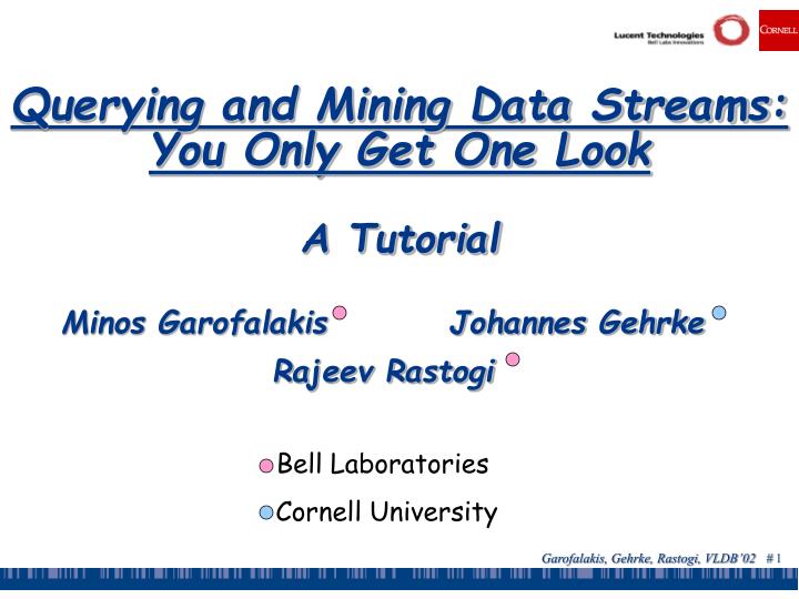
Querying and Mining Data Streams: You Only Get One Look A Tutorial. Minos Garofalakis Johannes Gehrke Rajeev Rastogi Bell Laboratories Cornell University. Outline. Introduction & Motivation Stream computation model, Applications Basic stream synopses computation

E N D
Querying and Mining Data Streams: You Only Get One LookA Tutorial Minos Garofalakis Johannes Gehrke Rajeev Rastogi Bell Laboratories Cornell University
Outline • Introduction & Motivation • Stream computation model, Applications • Basic stream synopses computation • Samples, Equi-depth histograms, Wavelets • Mining data streams • Decision trees, clustering, association rules • Sketch-based computation techniques • Self-joins, Joins, Wavelets, V-optimal histograms • Advanced techniques • Sliding windows, Distinct values, Hot lists • Future directions & Conclusions
Processing Data Streams: Motivation • A growing number of applications generate streams of data • Performance measurements in network monitoring and traffic management • Call detail records in telecommunications • Transactions in retail chains, ATM operations in banks • Log records generated by Web Servers • Sensor network data • Application characteristics • Massive volumes of data (several terabytes) • Records arrive at a rapid rate • Goal: Mine patterns, process queries and compute statistics on data streams in real-time
Data Streams: Computation Model • A data stream is a (massive) sequence of elements: • Stream processing requirements • Single pass: Each record is examined at most once • Bounded storage: Limited Memory (M) for storing synopsis • Real-time: Per record processing time (to maintain synopsis) must be low Synopsis in Memory Data Streams Stream Processing Engine (Approximate) Answer
Network Management Application • Network Management involves monitoring and configuring network hardware and software to ensure smooth operation • Monitor link bandwidth usage, estimate traffic demands • Quickly detect faults, congestion and isolate root cause • Load balancing, improve utilization of network resources Network Operations Center Measurements Alarms Network
IP Network Measurement Data • IP session data (collected using Cisco NetFlow) • AT&T collects 100 GBs of NetFlow data each day! • AT&T collects 100 GB of NetFlow data per day! Source Destination DurationBytes Protocol 10.1.0.2 16.2.3.7 12 20K http 18.6.7.1 12.4.0.3 16 24K http 13.9.4.3 11.6.8.2 15 20K http 15.2.2.9 17.1.2.1 19 40K http 12.4.3.8 14.8.7.4 26 58K http 10.5.1.3 13.0.0.1 27 100K ftp 11.1.0.6 10.3.4.5 32 300K ftp 19.7.1.2 16.5.5.8 18 80K ftp
Network Data Processing • Traffic estimation • How many bytes were sent between a pair of IP addresses? • What fraction network IP addresses are active? • List the top 100 IP addresses in terms of traffic • Traffic analysis • What is the average duration of an IP session? • What is the median of the number of bytes in each IP session? • Fraud detection • List all sessions that transmitted more than 1000 bytes • Identify all sessions whose duration was more than twice the normal • Security/Denial of Service • List all IP addresses that have witnessed a sudden spike in traffic • Identify IP addresses involved in more than 1000 sessions
Data Stream Processing Algorithms • Generally, algorithms compute approximate answers • Difficult to compute answers accurately with limited memory • Approximate answers - Deterministic bounds • Algorithms only compute an approximate answer, but bounds on error • Approximate answers - Probabilistic bounds • Algorithms compute an approximate answer with high probability • With probability at least , the computed answer is within a factor of the actual answer • Single-pass algorithms for processing streams also applicable to (massive) terabyte databases!
Outline • Introduction & Motivation • Basic stream synopses computation • Samples: Answering queries using samples, Reservoir sampling • Histograms: Equi-depth histograms, On-line quantile computation • Wavelets: Haar-wavelet histogram construction & maintenance • Mining data streams • Sketch-based computation techniques • Advanced techniques • Future directions & Conclusions
Sampling: Basics • Idea: A small random sample S of the data often well-represents all the data • For a fast approx answer, apply “modified” query to S • Example: select agg from R where R.e is odd (n=12) • If agg is avg, return average of odd elements in S • If agg is count, return average over all elements e in S of • n if e is odd • 0 if e is even Data stream: 9 3 5 2 7 1 6 5 8 4 9 1 Sample S: 9 5 1 8 answer: 5 answer: 12*3/4 =9 • Unbiased: For expressions involving count, sum, avg: the estimator • is unbiased, i.e., the expected value of the answer is the actual answer
Probabilistic Guarantees • Example: Actual answer is within 5 ± 1 with prob 0.9 • Use Tail Inequalities to give probabilistic bounds on returned answer • Markov Inequality • Chebyshev’s Inequality • Hoeffding’s Inequality • Chernoff Bound
Tail Inequalities Probability distribution Tail probability • General bounds on tail probability of a random variable (that is, probability that a random variable deviates far from its expectation) • Basic Inequalities: Let X be a random variable with expectation and variance Var[X]. Then for any Markov: Chebyshev:
Tail Inequalities for Sums • Possible to derive stronger bounds on tail probabilities for the sum of independent random variables • Hoeffding’s Inequality: Let X1, ..., Xm be independent random variables with 0<=Xi <= r. Let and be the expectation of . Then, for any , • Application to avg queries: • m is size of subset of sample S satisfying predicate (3 in example) • r is range of element values in sample (8 in example) • Application to count queries: • m is size of sample S (4 in example) • r is number of elements n in stream (12 in example) • More details in [HHW97]
Tail Inequalities for Sums (Contd.) • Possible to derive even stronger bounds on tail probabilities for the sum of independent Bernoulli trials • Chernoff Bound: Let X1, ..., Xm be independent Bernoulli trials such that Pr[Xi=1] = p (Pr[Xi=0] = 1-p). Let and be the expectation of . Then, for any , • Application to count queries: • m is size of sample S (4 in example) • p is fraction of odd elements in stream (2/3 in example) • Remark: Chernoff bound results in tighter bounds for count queries compared to Hoeffding’s inequality
Computing Stream Sample • Reservoir Sampling [Vit85]:Maintains a sample S of a fixed-size M • Add each new element to S with probability M/n, where n is the current number of stream elements • If add an element, evict a random element from S • Instead of flipping a coin for each element, determine the number of elements to skip before the next to be added to S • Concise sampling [GM98]: Duplicates in sample S stored as <value, count> pairs (thus, potentially boosting actual sample size) • Add each new element to S with probability 1/T (simply increment count if element already in S) • If sample size exceeds M • Select new threshold T’ > T • Evict each element (decrement count) from S with probability 1-T/T’ • Add subsequent elements to S with probability 1/T’
Counting Samples [GM98] • Effective for answering hot list queries (k most frequent values) • Sample S is a set of <value, count> pairs • For each new stream element • If element value in S, increment its count • Otherwise, add to S with probability 1/T • If size of sample S exceeds M, select new threshold T’ > T • For each value (with count C) in S, decrement count in repeated tries until C tries or a try in which count is not decremented • First try, decrement count with probability 1- T/T’ • Subsequent tries, decrement count with probability 1-1/T’ • Subject each subsequent stream element to higher threshold T’ • Estimate of frequency for value in S: count in S + 0.418*T
Histograms • Histograms approximate the frequency distribution of element values in a stream • A histogram (typically) consists of • A partitioning of element domain values into buckets • A count per bucket B (of the number of elements in B) • Long history of use for selectivity estimation within a query optimizer [Koo80], [PSC84], etc. • [PIH96] [Poo97] introduced a taxonomy, algorithms, etc.
Types of Histograms • Equi-Depth Histograms • Idea: Select buckets such that counts per bucket are equal • V-Optimal Histograms [IP95] [JKM98] • Idea: Select buckets to minimize frequency variance within buckets Count for bucket 1 2 3 4 5 6 7 8 9 10 11 12 13 14 15 16 17 18 19 20 Domain values Count for bucket 1 2 3 4 5 6 7 8 9 10 11 12 13 14 15 16 17 18 19 20 Domain values
Answering Queries using Histograms [IP99] answer: 3.5 * • (Implicitly) map the histogram back to an approximate relation, & apply the query to the approximate relation • Example: select count(*) from R where 4 <= R.e <= 15 • For equi-depth histograms, maximum error: Count spread evenly among bucket values 1 2 3 4 5 6 7 8 9 10 11 12 13 14 15 16 17 18 19 20 4 R.e 15
Equi-Depth Histogram Construction • For histogram with b buckets, compute elements with rank n/b, 2n/b, ..., (b-1)n/b • Example: (n=12, b=4) Data stream: 9 3 5 2 7 1 6 5 8 4 9 1 After sort: 1 1 2 3 4 5 5 6 7 8 9 9 rank = 9 (.75-quantile) rank = 3 (.25-quantile) rank = 6 (.5-quantile)
Computing Approximate Quantiles Using Samples • Problem: Compute element with rank r in stream • Simple sampling-based algorithm • Sort sample S of stream and return element in position rs/n in sample (s is sample size) • With sample of size , possible to show that rank of returned element is in with probability at least • Hoeffding’s Inequality: probability that S contains greater than rs/n elements from is no more than • [CMN98][GMP97] propose additional sampling-based methods Stream: r Sample S: rs/n
Algorithms for Computing Approximate Quantiles • [MRL98],[MRL99],[GK01] propose sophisticated algorithms for computing stream element with rank in • Space complexity proportional to instead of • [MRL98], [MRL99] • Probabilistic algorithm with space complexity • Combined with sampling, space complexity becomes • [GK01] • Deterministic algorithm with space complexity
Single-Pass Quantile Computation Algorithm [MRL 98] • Split memory M into b buffers of size k (M = bk) • For each successive set of k elements in stream • If free buffer B exists • insert k elements into B, set level of B to 0 • Else • merge two buffers B and B’ at same level l • output result of merge into B’, set level of B’ to l+1 • insert k elements into B, set level of B to 0 • Output element in position r after making copies of each element in final buffer and sorting them • Merge operation (input buffers B and B’ at level l) • Make copies of each element in B and B’ • Sort copies • Output elements in positions in sorted sequence, j=0, ..., k-1
Single-Pass Algorithm (Example) • M=9, b=3, k=3, r =10 • Computed quantile (r=10) level = 2 1 3 7 1 1 1 1 3 3 5 5 7 7 8 8 1 3 7 1 2 3 5 7 9 1 5 8 level = 1 level = 0 4 9 1 6 5 8 9 3 5 2 7 1 1 1 1 1 3 3 3 3 7 7 7 7
Analysis of Algorithm • Number of elements that are neither definitely small, nor definately large: • Algorithm returns element with rank r’, where • Choose smallest b such that and bk = M b
Computing Approximate Quantiles [GK01] • Synopsis structure S: sequence of tuples • : min/max rank of • : number of stream elements covered by • Invariants: Sorted sequence
Computing Quantile from Synopsis • Theorem: Let i be the max index such that . Then,
Inserting a Stream Element into the Synopsis • Let v be the value of the stream element, and and be tuples in S such that • Maintains invariants • elements per value • for a tuple is never modified, after it is inserted Inserted tuple with value v
Overview of Algorithm & Analysis Maintain our error invariant • Theorem: Maximum number of “alive” tuples from each -band is • Overall space complexity: • Partition the values into “bands” • Remember: we need to maintain => tuples in higher bands have more capacity ( = max. no. of observations that can be counted in ) • Periodically (every observations) compress the quantile synopsis in a right-to-left pass • Collapse ti into t(i+1) if: (a) t(i+1) is at a higher -band than ti, and (b)
Bands • values split into bands • size of band (adjusted as n increases) • Higher bands have higher capacities (due to smaller values) • Maximum value of in band : • Number of elements covered by tuples with bands in [0, ..., ]: • elements per value Bands:
Tree Representation of Synopsis • Parent of tuple ti: closest tuple tj (j>i) with band(tj) > band(ti) • Properties: • Descendants of ti have smaller band values than ti (larger values) • Descendants of ti form a contiguous segment in S • Number of elements covered by ti (with band ) and descendants: • Note: gi* is sum of gi values of ti and its descendants • Collapse each tuple with parent or sibling in tree root Longest sequence of tuples with band less than band(ti)
Compressing the Synopsis • Every elements, compress synopsis • For i from s-1 down to 1 • delete ti and all its descendants from S • Maintains invariants: root
Analysis • Lemma: Both insert and compress preserve the invariant • Theorem: Let i be the max index in S such that . Then, • Lemma: Synopsis S contains at most tuples from each band • For each tuple ti in S, • Also, and • Theorem: Total number of tuples in S is at most • Number of bands:
One-Dimensional Haar Wavelets [1.5, 4] [0.5, 0] [2.75] [-1.25] Haar wavelet decomposition: [2.75, -1.25, 0.5, 0, 0, -1, -1, 0] • Wavelets: Mathematical tool for hierarchical decomposition of functions/signals • Haar wavelets: Simplest wavelet basis, easy to understand and implement • Recursive pairwise averaging and differencing at different resolutions Resolution Averages Detail Coefficients 3 [2, 2, 0, 2, 3, 5, 4, 4] ---- 2 [2, 1, 4, 4] [0, -1, -1, 0] 1 0
Haar Wavelet Coefficients 2.75 - 2.75 + -1.25 -1.25 - 0 -1 0.5 -1 0 0 + - 0.5 + 0 - + - + 0 + - -1 + - -1 + 0 • Hierarchical decomposition structure (a.k.a. “error tree”) Coefficient “Supports” + + - + - + - + - + - + - + - 2 2 0 2 3 5 4 4 Original frequency distribution
Wavelet-based Histograms [MVW98] • Problem: Range-query selectivity estimation • Key idea: Use a compact subset of Haar/linear wavelet coefficients for approximating frequency distribution • Steps • Compute cumulative frequency distribution C • Compute Haar (or linear) wavelet transform of C • Coefficient thresholding : only m<<n coefficients can be kept • Take largest coefficients in absolutenormalized value • Haar basis: divide coefficients at resolution j by • Optimal in terms of the overall Mean Squared (L2) Error • Greedy heuristic methods • Retain coefficients leading to large error reduction • Throw away coefficients that give small increase in error
Using Wavelet-based Histograms • Selectivity estimation: count(a<= R.e<= b) = C’[b] - C’[a-1] • C’ is the (approximate) “reconstructed” cumulative distribution • Time: O(min{m, logN}), where m = size of wavelet synopsis (number of coefficients), N= size of domain • Empirical results over synthetic data • Improvements over random sampling and histograms • At most logN+1 coefficients are needed to reconstruct any C’ value C’[a]
Dynamic Maintenance of Wavelet-based Histograms [MVW00] Change propagates up to the root coefficient • Build Haar-wavelet synopses on the original frequency distribution • Similar accuracy with CDF, makes maintenance simpler • Key issues with dynamic wavelet maintenance • Change in single distribution value can affect the values of many coefficients (path to the root of the decomposition tree) • As distribution changes, “most significant” (e.g., largest) coefficients can also change! • Important coefficients can become unimportant, and vice-versa
Effect of Distribution Updates • Key observation: for each coefficient c in the Haar decomposition tree • c = ( AVG(leftChildSubtree(c)) - AVG(rightChildSubtree(c)) ) / 2 + - + - • Only coefficients on path(v) are affected and each can be updated in constant time h
Maintenance Algorithm [MWV00] - Simplified Version • Histogram H: Top m wavelet coefficients • For each new stream element (with value v) • For each coefficient c on path(v) and with “height” h • If c is in H, update c (by adding or substracting ) • For each coefficient c on path(v) and not in H • Insert c into H with probability proportional to (Probabilistic Counting [FM85]) • Initial value of c: min(H), the minimum coefficient in H • If H contains more than m coefficients • Delete minimum coefficient in H
Outline • Introduction & motivation • Stream computation model, Applications • Basic stream synopses computation • Samples, Equi-depth histograms, Wavelets • Mining data streams • Decision trees, clustering • Sketch-based computation techniques • Self-joins, Joins, Wavelets, V-optimal histograms • Advanced techniques • Sliding windows, Distinct values, Hot lists • Future directions & Conclusions
Clustering Data Streams [GMMO01] K-median problem definition: • Data stream with points from metric space • Find k centers in the stream such that the sum of distances from data points to their closest center is minimized. Previous work: Constant-factor approximation algorithms Two-step algorithm: STEP 1: For each set of M records, Si, find O(k) centers in S1, …, Sl • Local clustering: Assign each point in Sito its closest center STEP 2: Let S’ be centers for S1, …, Sl with each center weighted by number of points assigned to it. Cluster S’ to find k centers Algorithm forms a building block for more sophisticated algorithms (see paper).
One-Pass Algorithm - First Phase (Example) 1 2 4 5 3 • M= 3, k=1, Data Stream: 1 2 4 5 3
One-Pass Algorithm - Second Phase (Example) 1 2 1 4 5 w=3 3 5 w=2 S’ • M= 3, k=1, Data Stream:
Analysis • Observation 1: Given dataset D and solution with cost C where medians do not belong to D, then there is a solution with cost 2C where the medians belong to D. • Argument: Let m be the old median. Consider m’ in D closest to the m, and a point p. • If p is closest to the median: DONE. • If is not closest to the median: d(p,m’) <= d(p,m) + d(m,m’) <= 2*d(p,m) 1 m’ 5 m p
Analysis: First Phase • Observation 2: The sum of the optimal solution costs for the k-median problem for S1, …, Sl is at most twice the cost of the optimal solution for S 1 1 cost S 2 2 4 4 5 cost S 3 3 Data Stream
Analysis: Second Phase • Observation 3: Cluster weighted medians S’ • Consider point x with median m* in S and median m in Si.Let m belong to median m’ in S’Cost due to x in S’ = d(m,m’) Note that d(m,m*) <= d(m,x) + d(x,m*) Optimal cost (with medians m* in S) <= sum cost(Si) + cost(S) • Use Observation 1 to construct solution for medians m’ in S’ with additional factor 2. m cost Si m’ x 5 cost S m*
Overall Analysis of Algorithm • Final Result:Cost of final solution is at most the sum of costs of S’ and S1, …, Sl, which is at most a constant times (8) cost of S • If constant factor approximation algorithm is used to cluster S1, …, Sl then simple algorithm yields constant factor approximation • Algorithm can be extended to cluster in more than 2 phases w=3 1 1 cost S’ cost 2 2 w=2 4 4 5 5 cost 3 3 Data Stream S’
Decision Trees Age Minivan YES <30 >=30 Sports,Truck YES Car Type YES NO Minivan Sports, Truck NO YES 0 30 60 Age
Decision Tree Construction • Top-down tree construction schema: • Examine training database and find best splitting predicate for the root node • Partition training database • Recurse on each child node BuildTree(Node t, Training database D, Split Selection Method S) (1) Apply S to D to find splitting criterion (2) if (t is not a leaf node) (3) Create children nodes of t (4) Partition D into children partitions (5) Recurse on each partition (6) endif