Download

1 / 30
410 likes | 662 Views
Least squares. CS1114 http://cs1114.cs.cornell.edu. Robot speedometer. Suppose that our robot can occasionally report how far it has traveled (mileage) How can we tell how fast it is going? This would be a really easy problem if: The robot never lied

E N D
Least squares CS1114 http://cs1114.cs.cornell.edu
Robot speedometer • Suppose that our robot can occasionally report how far it has traveled (mileage) • How can we tell how fast it is going? • This would be a really easy problem if: • The robot never lied • I.e., it’s mileage is always exactly correct • The robot travels at the same speed • Unfortunately, the real world is full of lying, accelerating robots • We’re going to figure out how to handle them
Speedometer approach • We are (as usual) going to solve a very general version of this problem • And explore some cool algorithms • Many of which you will need in future classes • The velocity of the robot at a given time is the change in mileage w.r.t. time • For our ideal robot, this is the slope of the line • The line fits all our data exactly • In general, if we know mileage as a function of time, velocity is the derivative • The velocity at any point in time is the slope of the mileage function
Estimating velocity • So all we need is the mileage function • We have as input some measurements • Mileage, at certain times • A mileage function takes as input something we have no control over • Input (time): independent variable • Output (mileage): dependent variable Dependent variable (mileage) Independent variable (time)
Basic strategy • Based on the data, find mileage function • From this, we can compute: • Velocity (1st derivative) • Acceleration (2nd derivative) • For a while, we will only think about mileage functions which are lines • In other words, we assume lying, non-accelerating robots • Lying, accelerating robots are much harder
Models and parameters • A model predicts a dependent variable from an independent variable • So, a mileage function is actually a model • A model also has some internal variables that are usually called parameters • In our line example, parameters are m,b Parameters (m,b) Dependent variable (mileage) Independent variable (time)
Linear regression • Simplest case: fitting a line
Linear regression • Simplest case: just 2 points (x2,y2) (x1,y1)
Linear regression • Simplest case: just 2 points • Want to find a line y = mx + b • x1 y1, x2 y2 • This forms a linear system: y1 = mx1 + b y2 = mx2 + b • x’s, y’s are knowns • m, b are unknown • Very easy to solve (x2,y2) (x1,y1)
Linear regression, > 2 points • The line won’t necessarily pass through any data point (yi, xi) y = mx + b
Some new definitions • No line is perfect – we can only find the best line out of all the imperfect ones • We’ll define an objective function Cost(m,b) that measures how far a line is from the data, then find the best line • I.e., the (m,b) that minimizes Cost(m,b)
Line goodness • What makes a line good versus bad? • This is actually a very subtle question
Residual errors • The difference between what the model predicts and what we observe is called a residual error (i.e., a left-over) • Consider the data point (x,y) • The model m,b predicts (x,mx+b) • The residual is y – (mx + b) • For 1D regressions, residuals can be easily visualized • Vertical distance to the line
Least squares fitting This is a reasonable cost function, but we usually use something slightly different
Least squares fitting We prefer to make this a squared distance Called “least squares”
Why least squares? • There are lots of reasonable objective functions • Why do we want to use least squares? • This is a very deep question • We will soon point out two things that are special about least squares • The full story probably needs to wait for graduate-level courses, or at least next semester
Gradient descent • Basic strategy: • Start with some guess for the minimum • Find the direction of steepest descent (gradient) • Take a step in that direction (making sure that you get lower, if not, adjust the step size) • Repeat until taking a step doesn’t get you much lower
Gradient descent, 1D quadratic • There is some magic in setting the step size
Some error functions are easy • A (positive) quadratic is a convex function • The set of points above the curve forms a (infinite) convex set • The previous slide shows this in 1D • But it’s true in any dimension • A sum of convex functions is convex • Thus, the sum of squared error is convex • Convex functions are “nice” • They have a single global minimum • Rolling downhill from anywhere gets you there
Consequences • Our gradient descent method will always converge to the right answer • By slowly rolling downhill • It might take a long time, hard to predict exactly how long (see CS3220 and beyond)
Why is an error function hard? • An error function where we can get stuck if we roll downhill is a hard one • Where we get stuck depends on where we start (i.e., initial guess/conditions) • An error function is hard if the area “above it” has a certain shape • Nooks and crannies • In other words, CONVEX! • Non-convex error functions are hard to minimize
What else about LS? • Least squares has an even more amazing property than convexity • Consider the linear regression problem • There is a magic formula for the optimal choice of (m,b) • You don’t need to roll downhill, you can “simply” compute the right answer
Closed-form solution! • This is a huge part of why everyone uses least squares • Other functions are convex, but have no closed-form solution
Closed form LS formula • The derivation requires linear algebra • Most books use calculus also, but it’s not required (see the “Links” section on the course web page) • There’s a closed form for any linear least-squares problem
Linear least squares • Any formula where the residual is linear in the variables • Examples linear regression: [y – (mx + b)]2 • Non-example: [x’ – abc x]2 (variables: a, b, c)
Linear least squares • Surprisingly, fitting the coefficients of a quadratic is still linear least squares • The residual is still linear in the coefficients β1, β2, β3 Wikipedia, “Least squares fitting”
Optimization • Least squares is another example of an optimization problem • Optimization: define a cost function and a set of possible solutions, find the one with the minimum cost • Optimization is a huge field
Sorting as optimization • Set of allowed answers: permutations of the input sequence • Cost(permutation) = number of out-of-order pairs • Algorithm 1: Snailsort • Algorithm 2: Bubble sort • Algorithm 3: ???