Download
1 / 15
170 likes | 281 Views
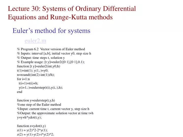
Lecture 30: Systems of Ordinary Differential Equations and Runge-Kutta methods. Euler’s method for systems. euler2.m. % Program 6.2 Vector version of Euler method % Inputs: interval [a,b], initial vector y0, step size h % Output: time steps t, solution y

E N D
Lecture 30: Systems of Ordinary Differential Equations and Runge-Kutta methods Euler’s method for systems euler2.m % Program 6.2 Vector version of Euler method % Inputs: interval [a,b], initial vector y0, step size h % Output: time steps t, solution y % Example usage: [t y]=euler2([0 1],[0 1],0.1); function [t y]=euler2(int,y0,h) t(1)=int(1); y(1,:)=y0; n=round((int(2)-int(1))/h); for i=1:n t(i+1)=t(i)+h; y(i+1,:)=eulerstep(t(i),y(i,:),h); end function y=eulerstep(t,y,h) %one step of the Euler method %Input: current time t, current vector y, step size h %Output: the approximate solution vector at time t+h y=y+h*ydot(t,y); function z=ydot(t,y) z(1) = y(2)^2-2*y(1); z(2) = y(1)-y(2)-t*y(2)^2;
%euler2test.m - test of function euler2. Runing require file euler2.m % Example usage: y=euler2([0 1],[0 1],0.1); y1exact=inline('t.*exp(-2*t)'); y2exact=inline('exp(-t)'); [t y]=euler2([0 1], [0 1], 0.01); plot(t,y(:,1),t,y(:,2)); legend('y1','y2') y1exactvec=y1exact(t); y2exactvec=y2exact(t); ii=1:10; hvec=0.1./2.^ii; for i=1:length(hvec) [t y]=euler2([0 1], [0 1], hvec(i)); disp(['h=',num2str(hvec(i)),' Error in eulers method for y(1) =', num2str(y(length(y))-y1exactvec(length(y1exactvec)))]); end
>> euler2test h=0.05 Error in eulers method for y(1) =0.0057103 h=0.025 Error in eulers method for y(1) =0.0028366 h=0.0125 Error in eulers method for y(1) =0.0014133 h=0.00625 Error in eulers method for y(1) =0.00070534 h=0.003125 Error in eulers method for y(1) =0.00035234 h=0.0015625 Error in eulers method for y(1) =0.00017609 h=0.00078125 Error in eulers method for y(1) =8.8023e-005 h=0.00039063 Error in eulers method for y(1) =4.4006e-005 h=0.00019531 Error in eulers method for y(1) =2.2002e-005 h=9.7656e-005 Error in eulers method for y(1) =1.1001e-005
Euler’s method for system of 4 equations: Orbital motion around sun orbit.m
%Program 6.4 Plotting program for one-body problem % Inputs: int=[a b] time interval, initial conditions % ic = [x0 vx0 y0 vy0], x position, x velocity, y pos, y vel, % h = stepsize, p = steps per point plotted % Calls a one-step method such as trapstep.m % Example usage: orbit([0 100],[0 1 2 0],0.01,5) function z=orbit(int,ic,h,p) n=round((int(2)-int(1))/(p*h)); % plot n points x0=ic(1);vx0=ic(2);y0=ic(3);vy0=ic(4); % grab initial conds y(1,:)=[x0 vx0 y0 vy0];t(1)=int(1); % build y vector set(gca,'XLim',[-5 5],'YLim',[-5 5],'XTick',[-5 0 5],'YTick',... [-5 0 5],'Drawmode','fast','Visible','on','NextPlot','add'); cla; sun=line('color','y','Marker','.','markersize',25,... 'xdata',0,'ydata',0); drawnow; head=line('color','r','Marker','.','markersize',25,... 'erase','xor','xdata',[],'ydata',[]); tail=line('color','b','LineStyle','-','erase','none',... 'xdata',[],'ydata',[]); %[px,py,button]=ginput(1); % include these three lines %[px1,py1,button]=ginput(1); % to enable mouse support %y(1,:)=[px px1-px py py1-py]; % 2 clicks set direction for k=1:n for i=1:p t(i+1)=t(i)+h; y(i+1,:)=eulerstep(t(i),y(i,:),h); end y(1,:)=y(p+1,:);t(1)=t(p+1); set(head,'xdata',y(1,1),'ydata',y(1,3)) set(tail,'xdata',y(2:p,1),'ydata',y(2:p,3)) drawnow; End
function y=eulerstep(t,x,h) %one step of the Euler method y=x+h*ydot(t,x); function z = ydot(t,x) m2=3;g=1;mg2=m2*g;px2=0;py2=0; px1=x(1);py1=x(3);vx1=x(2);vy1=x(4); dist=sqrt((px2-px1)^2+(py2-py1)^2); z=zeros(1,4); z(1)=vx1; z(2)=(mg2*(px2-px1))/(dist^3); z(3)=vy1; z(4)=(mg2*(py2-py1))/(dist^3);
>> orbit([0 100], [0 1 2 0],0.01,5) Show animation
Orbital motion around sun but now with trapezoid method orbittrap.m %obrittrap. - using trapezoid method for integration % Inputs: int=[a b] time interval, initial conditions % ic = [x0 vx0 y0 vy0], x position, x velocity, y pos, y vel, % h = stepsize, p = steps per point plotted % Calls a one-step method such as trapstep.m % Example usage: orbittrap([0 100],[0 1 2 0],0.01,5) function z=orbit(int,ic,h,p) n=round((int(2)-int(1))/(p*h)); % plot n points x0=ic(1);vx0=ic(2);y0=ic(3);vy0=ic(4); % grab initial conds y(1,:)=[x0 vx0 y0 vy0];t(1)=int(1); % build y vector set(gca,'XLim',[-5 5],'YLim',[-5 5],'XTick',[-5 0 5],'YTick',... [-5 0 5],'Drawmode','fast','Visible','on','NextPlot','add'); cla; sun=line('color','y','Marker','.','markersize',25,... 'xdata',0,'ydata',0); drawnow; head=line('color','r','Marker','.','markersize',25,... 'erase','xor','xdata',[],'ydata',[]); tail=line('color','b','LineStyle','-','erase','none',... 'xdata',[],'ydata',[]); %[px,py,button]=ginput(1); % include these three lines %[px1,py1,button]=ginput(1); % to enable mouse support %y(1,:)=[px px1-px py py1-py]; % 2 clicks set direction
for k=1:n for i=1:p t(i+1)=t(i)+h; y(i+1,:)=trapstep(t(i),y(i,:),h); end y(1,:)=y(p+1,:);t(1)=t(p+1); set(head,'xdata',y(1,1),'ydata',y(1,3)) set(tail,'xdata',y(2:p,1),'ydata',y(2:p,3)) drawnow; end function y = trapstep(t,x,h) %one step of the Trapezoid Method z1=ydot(t,x); g=x+h*z1; z2=ydot(t+h,g); y=x+h*(z1+z2)/2; function z = ydot(t,x) m2=3;g=1;mg2=m2*g;px2=0;py2=0; px1=x(1);py1=x(3);vx1=x(2);vy1=x(4); dist=sqrt((px2-px1)^2+(py2-py1)^2); z=zeros(1,4); z(1)=vx1; z(2)=(mg2*(px2-px1))/(dist^3); z(3)=vy1; z(4)=(mg2*(py2-py1))/(dist^3);
>> orbittrap([0 100], [0 1 2 0],0.01,5) Show animation
Hodgkin-Huxley equations as example or 4th order Runge-Kutta method use
% Program 6.5 Hodgkin-Huxley equations % Inputs: [a b] time interval, % ic = initial voltage v and 3 gating variables, step size h % Output: solution y % Calls a one-step method such as rk4step.m % Example usage: y=hh([0 100],[-65 0 0.3 0.6],0.05); function y=hh(inter,ic,h) global pa pb pulse inp=input('pulse start, end, muamps in [ ], e.g. [50 51 7]: '); pa=inp(1);pb=inp(2);pulse=inp(3); a=inter(1);b=inter(2);n=ceil((b-a)/h); % plot n points in total y(1,:)=ic; % initial conditions t(1)=a; for i=1:n t(i+1)=t(i)+h; y(i+1,:)=rk4step(t(i),y(i,:),h); end subplot(3,1,1); plot([a pa pa pb pb b],[0 0 pulse pulse 0 0]); grid;axis([0 100 0 2*pulse]) ylabel('input pulse') subplot(3,1,2); plot(t,y(:,1));grid;axis([0 100 -100 100]) ylabel('voltage (mV)') subplot(3,1,3); plot(t,y(:,2),t,y(:,3),t,y(:,4));grid;axis([0 100 0 1]) ylabel('gating variables') legend('m','n','h') xlabel('time (msec)') hh.m
function y=rk4step(t,w,h) %one step of the Runge-Kutta order 4 method s1=ydot(t,w); s2=ydot(t+h/2,w+h*s1/2); s3=ydot(t+h/2,w+h*s2/2); s4=ydot(t+h,w+h*s3); y=w+h*(s1+2*s2+2*s3+s4)/6; function z = ydot(t,w) global pa pb pulse c=1;g1=120;g2=36;g3=0.3;T=(pa+pb)/2;len=pb-pa; e0=-65;e1=50;e2=-77;e3=-54.4; in=pulse*(1-sign(abs(t-T)-len/2))/2; % square pulse input on interval [pa,pb] of pulse muamps v=w(1);m=w(2);n=w(3);h=w(4); z=zeros(1,4); z(1)=(in-g1*m*m*m*h*(v-e1)-g2*n*n*n*n*(v-e2)-g3*(v-e3))/c; v = v-e0; z(2)=(1-m)*(2.5-0.1*v)/(exp(2.5-0.1*v)-1)-m*4*exp(-v/18); z(3)=(1-n)*(0.1-0.01*v)/(exp(1-0.1*v)-1)-n*0.125*exp(-v/80); z(4)=(1-h)*0.07*exp(-v/20) - h/(exp(3-0.1*v)+1);
Current above threshold 6.9: [50 51 7] >> hh([0 100],[-65 0 0.3 0.6],0.05) pulse start, end, muamps in [ ], e.g. [50 51 7]: [50 51 7]
Current below threshold 6.9: [50 51 5] >> hh([0 100],[-65 0 0.3 0.6],0.05) pulse start, end, muamps in [ ], e.g. [50 51 7]: [50 51 5]