Download
1 / 19
190 likes | 438 Views
The mystery of the CHI SQUARE. Is it CHEE square Or CHAI Square?!. Chi Square X 2 goodness of fit. There is a single test that can be applied to see if the observed sample distribution is significantly different in some way from the hypothesized population distribution.

E N D
The mystery of the CHI SQUARE • Is it CHEE square • Or • CHAI Square?!
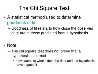
Chi SquareX2 goodness of fit There is a single test that can be applied to see if the observed sample distribution is significantly different in some way from the hypothesized population distribution
Accidents on Cellphones Are you more likely to have a motor vehicle collision when using a cell phone? A study of 699 drivers who were using a cell phone when they were involved in a collision examined this question. These drivers made 26,798 cell phone calls during a 14-month study period. Each of the 699 collisions was classified in various ways. Here are the counts for each day of the week:
Hypotheses: H0: Motor vehicle accidents involving cell phone use are equally likely to occur on each of the seven days of the week. Ha: The probabilities of a motor vehicle accident involving cell phone use vary from day to day (that is, they are not all the same).
Chi square procedure: In general, the expected count for any categorical variable is obtained by multiplying the proportion of the distribution for each category by the sample size.
For Sunday: For Monday: Chi-square test statistics
Finding the p-value Degrees of freedom: n-1 df: 7-1 = 6 Calculator syntax: 2nd - VARS - 8 (enter) X2 cdf( test statistic, 1E99, df ) X2 cdf( 208.84, 1E99, 6 ) p= 2.48 x 10-42
Conclusion H0: Motor vehicle accidents involving cell phone use are equally likely to occur on each of the seven days of the week. Ha: The probabilities of a motor vehicle accident involving cell phone use vary from day to day (that is, they are not all the same). Since the p value is extremely small (p= 2.48 x 10-42), there is sufficient evidence to reject H0 and conclude that these types of accidents are not equally likely to occur on each of the seven days of the week.
Red Eye Fruit Fly Any offspring receiving an R gene will have red eyes, and any offspring receiving a C gene will have straight wings. So based on this Punnett square, the biologists predict a ratio of 9 red-eyed, straight-winged (x) : 3 red-eyed, curly-winged (y) : 3 white-eyed, straight-winged (z) : 1 white-eyed, curly-winged (w) offspring. To test their hypothesis about the distribution of offspring, the biologists mate the fruit flies. Of 200 offspring, 99 had red eyes and straight wings, 42 had red eyes and curly wings, 49 had white eyes and straight wings, and 10 had white eyes and curly wings. Do these data differ significantly from what the biologists have predicted?
Given Distribution Ho: these proportions is correct for the the offspring of 2 parents Ha: at least one of these proportions is incorrect
Conditions and calculations: We can use a chi-square goodness of fit test to measure the strength of the evidence against the hypothesized distribution, provided that the expected cell counts are large enough. p=0.1029 X2 cdf(6.187, 1E99, 3 )
Interpretations The P-value of 0.1029 indicates that the probability of obtaining a sample of 200 fruit fly offspring in which the proportions differ from the hypothesized values by at least as much as the ones in our sample is over 10%, assuming that the null hypothesis is true. This is not sufficient evidence to reject the biologists' predicted distribution.
Your Turn Course grades Most students in a large college statistics course are taught by teaching assistants (TAs). One section is taught by the course supervisor, a full-time professor. The distribution of grades for the hundreds of students taught by TAs this semester was The grades assigned by the professor to the 91 students in his section were (a) What percents of students in the professor's section earned A, B, C, and D/F? In what ways does this distribution of grades differ from the TA distribution? (b) Because the TA distribution is based on hundreds of students, we are willing to regard it as a fixed probability distribution. If the professor's grading follows this distribution, what are the expected counts of each grade in his section? (c) Does the chi-square test for goodness of fit give good evidence that the professor's grade distribution differs from the TA distributions? Use the Inference Toolbox.
Answers: (a)“A”: 24.2%, “B”: 41.8%, “C”: 22.0%, “D/F”: 12.1%. Fewer A′ s and more D/F′ s than the TA sections. (b)“A”: 29.12, “B”: 37.31, “C”: 18.20, “D/F”: 6.37. (c)H0: p1 = 0.32, p1 = 0.41, p1 = 0.20, p1 = 0.07 vs. Ha: at least one of these proportions is different. All the expected counts are greater than 5, so the condition for X2 is satisfied. X2 = 5.297 (df = 3), so the P–value = 0.1513; there is not enough evidence to conclude that the professor′ s grade distribution was different from the TA grade distribution.
Chi-Sq. Practice (with probability model) Thai, the manager of a car dealership, did not want to stock cars that were bought less frequently because of their unpopular color. The five colors that he ordered were red, yellow, green, blue, and white. According to Thai,the expected frequencies or number of customers choosing each color should follow the percentages of last year. She felt 20% would choose yellow, 30% would choose red, 10% would choose green, 10% would choose blue, and 30% would choose white. She now took a random sample of 150 customers and asked them their color preferences.
Hypotheses: Ho: there is no significant difference between the proportion of the costumer’s car color preferences. Ho: p1 = p2 = p3 = p4 = p5 Ha:there is a significant difference between the proportion of the costumer’s car color preferences. Ha: p1 ≠ p2 ≠ p3 ≠ p4 ≠ p5
Chi-square procedure: X2= 26.95 P-value = 2.03x10⁻⁵
Conclusion Since our p-value is small, we have sufficient reason to reject the null hypothesis making our test significant. Therefore,there is a significant difference between the proportion of the costumer’s car color preferences.